*
Corresponding author
Few heuristic optimization algorithms to solve the multi-period fixed
charge production-distribution problem
N. Balajia,* and N. Jawaharb
a
Department of Mechanical Engineering,Sri Krishna College of Engineering and Technology, Coimbatore 641 008, India.
b
Department of Mechanical Engineering, Thiagarajar College of Engineering, Madurai 625 015, India.
Article info:
Received: 05/09/2011 Accepted: 22/11/2011 Online: 03/03/2012
Keywords:
Multi-period fixed charge problem,
0-1 mixed integer programming problem, Genetic algorithm, Simulated annealing algorithm,
Equivalent variable cost
Abstract
This paper deals with a multi-period fixed charge production-distribution problem associated with backorder and inventories. The objective is to determine the size of the shipments from each supplier and backorder and inventories at each period, so that the total cost incurred during the entire period towards production, transportation, backorder and inventories is minimised. A 0-1 mixed integer programming problem is formulated.
Genetic algorithm based population search heuristic, Simulated annealing based neighbourhood search heuristic and Equivalent variable cost based simple heuristic are proposed to solve the formulation. The proposed methodologies are evaluated by comparing their solutions with the lower bound solutions. The comparisons reveal that Genetic algorithm and Simulated annealing algorithm generate better solutions than the Equivalent variable cost solutions and are capable of providing solutions close to the lower bound value of the problems.
1. Introduction
In a scattered production system, the production location also determines the overall production costs. It is because, the urban location will require more labour and overhead costs than rural location. Moreover, in such scattered production system with scattered customers, the production location influences the distribution schedule and thereby distribution costs. Therefore, in industrial problems where production and distribution costs are both of a
inventories in the distribution channel. As a result of this pressure, many companies are exploring closer coordination along the manufacturing/ distribution channel [2]. Many companies strive to synchronize their production, transportation and replenishment planning by adopting supply chain management practices such as vendor-managed inventory, efficient consumer response, and collaborative planning, forecasting and replenishment. The main objective of these collaborative methods is to reduce inefficiencies and to eliminate redundancies between the different partners [3]. The multi-period fixed charge production-distribution problem (MPFCPDP) is an extension of FCT (fixed charge transportation) problem, where the time based strategic decisions on size of the shipments from each supplier, inventory, and backorder can make an economical distribution. The MPFCPDP problem is difficult to solve due to the presence of fixed costs, which cause nonlinearities in the objective function and are known to be Non-deterministic Polynomial-time ‘NP’ hard [4]. The complexity of the problem is further increased, when supplier dependent product cost, time dependent inventory and backorder are included in the model. This limits the usage of the conventional multi-period and fixed charge solution procedures.
There are many different multi-period distribution problems (MPDP) in the literature [2, 3, 5-12] involving considerations of production and transportation, possibly together with other functions. The review on multi-period problems reveals the following: most of the models attempt to integrate inventory and transportation issues; excess in availability in any period is held as inventory at the suppliers end and is used for the subsequent periods; inventory at the demand points has not been given due consideration; admission of backorder may considerably reduce the total cost of logistics; not all the papers (except [6,8,10]) have included the fixed charge associated with transportation; though few papers have included fixed charge in their models, they do not deal exactly the multi-period fixed charge production-distribution between multiple sources (suppliers) and
multiple destinations (customers) with inventory alternatives and backorder consideration to optimize the total production-distribution cost.
In the light of the above, this paper considers a MPFCPDP problem concerning the production, transportation and storage of finished goods from ‘m’ suppliers (industrial producers) to ‘n’ customers (demand centers like assembling centers, distribution centers etc.). The transportation cost is the main element in the proposed production-distribution model. The other considerations are storage and backorders. This paper considers a two-echelon inventory system where the suppliers’ supply capacity and customers’ demands are deterministic. The purpose of maintaining two-echelon inventory is to minimize the total distribution cost while integrating production, transportation, backorder and inventories. The production-distribution planning problem addressed here as MPFCPDP, is formulated as a 0-1 mixed integer programming problem. Genetic algorithm (GA) based population search heuristic, Simulated annealing algorithm (SAA) based neighbourhood search heuristic and an Equivalent variable cost (EVC) based simple heuristic are proposed to solve the formulation. The rest of the paper is organised as follows: Section 2 addresses the problem environment and mathematical formulation of the MPFCPDP. Section 3 discusses about the proposed heuristics. Section 4 provides a numerical illustration. Section 5 discusses the computational results and performance analysis of the proposed methodologies. A summary of the present analysis and future research directions are presented in the concluding section 6.
2. Problem environment and description
supplier i can produce the product at a production cost of CUi per unit and ship it to any customer j at a transportation cost of Cij per unit for shipping from supplier i to customer j plus a fixed cost of FCij included for operating the route i to j. At any time period t, the total cumulative production of the suppliers may or may not be equal to the total demand of the customers. The excess or shortage of production in the period t is carried over to the subsequent period t+1. The excess of production in period t, addressed here as the inventory, is considered as an additional supply available for the period t+1. It is notified as SIit at an inventory holding cost of SHi per unit per period at ith supplier’s location and CIjt at an inventory holding cost of CHj per unit per period at jth customer’s location. On the other hand, the production shortage of the period t (excess demand), addressed here as backorder, is considered as an additional demand for the period t+1. It is notified as BLj
t
at a penalty cost of BCj per unit per period at j
th
customer’s location. As the proposed model considers short planning periods (days/weeks/months), the cost associated with production (CUi), transportation (i.e. Cij and FCij), inventory (i.e. SHi and CHj) and backorder (i.e. BCj) are independent of period t. The beginning period’s inventory and backorder (i.e., SIi
0 , CIj
0
and BLj 0
) are known quantities. Minimization of the sum of costs of production, transportation, holding inventory and penalty for the backorder supply is considered as the objective criterion of the problem.
3. Decision variables
Xij :Number of units of shipments from supplier i to customer j in period t
SIi t
:Number of units of inventory with supplier i in period t
CIj t
:Number of units of inventory with customer j in period t
BLjt :Number of units of backlog for customer j in period t
ij t
:Binary variable that specifies the product distribution from supplier i to customer j in period t (i.e., ij
t
= 1 if Xij t
> 0 and
ijt = 0 if Xijt = 0)
4. Mathematical model
This model attempts to integrate production, transportation, backorder and inventory decisions monolithically from a centralized planning point of view. Let ijt be a binary
variable to account fixed transportation cost. The mathematical model of the MPFCPDP problem is formulated as a 0-1 Mixed Integer Programming (MIP) problem as given below.
1 1 1 1 1 1 * * T t n j T t n j t j j t jj CI BC BL
CH (1)
Subject to :
t i n j t ij t i t
i SI X SI
P
1 1
i , i=1… m & t , t=1…T; (2)
m i t j t j t ij t j t j tj BL CI X BL CI
D
1 1 1
j , j=1… n & t , t=1…T; (3)
0; > if 1 ijt t
ij X
i , i=1… m, j , j=1… n & t , t=1…T; (4)
0; if 0 t ij t ij X
i , i=1… m, j , j=1… n & t , t=1…T;
(5) 0 t ij X
i , i=1… m, j , j=1… n & t , t=1…T;
(6)
0
t i
SI and integer;
i , i=1… m, & t , t=1…T; (7)
0
t j CI
and integer;
j , j=1… n & t , t=1…T; (8)
0
t j
BL and integer;
j , j=1… n & t , t=1…T; (9)
The objective function given by Eq. (1) aims to minimize the sum of the total costs associated with production, transportation, inventory at supplier’s side and customer’s side and backorder. The first term of the objective function provides the total cost of production for the entire period T and the second term provides the total cost of transportation for the entire period T. The third term addresses the total cost of holding inventory at supplier’s locations for the entire period T. The fourth and the fifth terms indicate respectively the total cost holding inventory for the entire period T and the total cost of backorder penalty for the entire period T. Constraint set given by Eq. (2) expresses the material balance at the supplier’s side between any two successive time intervals. Similarly, constraint set (3) expresses the material balance at the customer’s side between any two successive time intervals. In the left and right sides of the constraint set 3, either the inventory or backorder is present. Constraint sets given by Eqs. (4) and (5) return a binary value of ijt depending on the value of Xijt. Constraint sets given by Eqs. (6) to (9) ensure the non-negativity nature of decision variables Xijt, SIit, CIjt, and BLjt.
5. Solution methodologies
In this paper, the MPFCPDP modelis solved by GA and SAA based meta-heuristics and EVC based simple heuristics. They are delineated in the following sections.
5.1. GA and SAA based meta-heuristics
Over the last thirty years, there has been a growing interest in problem solving systems based on the principles of population based and neighborhood based search heuristics. In population based search heuristics, the GA has been increasingly applied to various search and optimization problems and has emerged as potential techniques to provide solutions with acceptable accuracy for NP hard problems [13-15]. In neighborhood based search heuristics, many researchers considered SAA for solving many hard optimisation problems [15-20]. The proposed GA and SAA based heuristics are structured to solve the MPFCPDP in two stages. They are as follows.
Stage I: Data input and transformation
This stage remains common in both GA and SAA based heuristics. It accepts the data of MPFCPDP under consideration as input and modulates them as a single-period fixed charge production-distribution problem (SPFCPDP) data set. The conversion provides a modulated data suitable for allocating the shipment quantities in single-period layout and subsequently deriving a feasible multi-period distribution schedule in the following GA and SAA routines, which is delineated in Stage II.
Stage II: Procedural steps of GA Step 1: Parameters setting The parameters of GA are:
pop_size
= 10;p_cross
= 0.5; p_mut = 0.1;Step 2: Initial population generation
In this proposed GA, a chromosome
c
refers to a gene type representation of a distribution schedule to the SPFCPDP. The chromosomec
is the permutation of cell numbers of SPFCPDP matrix, in which each cell is identified with a unique The total number of cells in the SPFCPDP, which is also equal to the length of the chromosomec
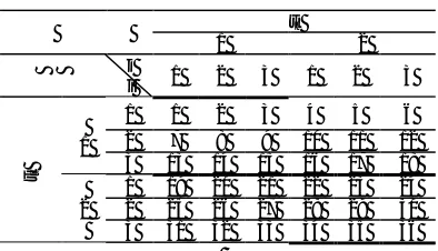
, thus becomes (m*T)*(n*T). When the supply and demand are in same period (i.e. tc = tr), then they form T number of diagonal matrix of size m*n. The number of cells in the diagonal matrix thus becomes equal to m*n*T. Table 1 illustrates an example (m*n*T: 3*3*2) SPFCPDP matrix cell numbers.A chromosome is structured as two parts. The first part is framed by the cell numbers of diagonal SPFCPDP matrix. The second part is framed by the remaining cell numbers of non-diagonal SPFCPDP matrix. Table 2 shows a randomly developed chromosome with cell number for the above example. In the same way, a randomly developed ten chromosomes form the initial population.
Table 1. SPFCPDP cell numbers matrix.
tc
1 2
j
i 1 2 3 1 2 3
tr
1
1 1 2 3 4 5 6 2 7 8 9 10 11 12 3 13 14 15 16 17 18
2
1 19 20 21 22 23 24 2 25 26 27 28 29 30 3 31 32 33 34 35 36
Table 2. An example chromosome of SPFCPDP.
First part
Cell number
1 2 3 4 5 6 7 8 9 10 11 12 13 14 15 16 17 18 34 23 7 3 22 9 30 13 1 28 8 15 35 2 14 24 36 29
Sec. part
Cell number
28 29 30 31 32 33 34 35 36 37 38 39 40 41 42 43 44 45
18 5 26 10 6 27 16 4 17 31 25 32 12 19 11 21 20 33
Step 3: Evaluation
The chromosome, on decoding, provides a feasible distribution schedule to the MPFCPDP by allocating shipment quantities to the cells of SPFCPDP based on their priority as per the cell number positions in the chromosome. Then the actual MPFCPDP distribution quantities Xijt, suppliers’ inventory SIit, customers’ inventory
CIjt, and backlog BLjt are derived by demodulating the allocations of SPFCPDP. The total production-distribution cost Z(m) corresponding to MPFCPDP distribution schedule (m) is calculated from the objective Eq. (1). Each chromosome
c
in the initial population is evaluated in terms of Z by the same procedure.Step 4: Updating
At the end of first generation, the followings parameters are updated.
t global_bes best
pop_
. 1
gen_no gen_no
Step 5: Termination checking:
The number of generations is considered as the termination criterion. The termination criterion value of the illustration is calculated as follows. Termination criterion = n_gen =100+ (m*T)*(n*T). If the gen_no value is less than
n_gengo to the next step, else go to step 7.
Step 6: New population generation
Step 7: Output
The distribution schedule ((best)) and distribution cost (Z(near opt)) in the global_best are the solutions to the problem and are given as output.
Stage II: Procedural steps of SAA
Step 1: Initialization of SAA parameters and counters
The parameters of SAA are:
TE = 475, ACCEPT = 0, TOTAL = 0, FREEZE = 0, α =0.90 and
Termination condition = (FREEZE = 5 or TE = 20).
Step 2: Generation of initial seed string
In this proposed SAA, a string S refers to a gene type representation of a distribution schedule to the SPFCPDP. The string S is the permutation of cell numbers of SPFCPDP matrix, in which each cell is identified with a unique The total number of cells in the SPFCPDP, which is also equal to the length of the string S, thus becomes (m*T)*(n*T). When the supply and demand are in same period (i.e. tc = tr), then they form T number of diagonal matrix of size m*n. The number of cells in the diagonal matrix thus becomes equal to m*n*T. Table 3 illustrates an example (m*n*T: 3*3*2) of SPFCPDP matrix cell numbers.
Table 3. SPFCPDP cell numbers matrix.
tc
1 2
j
i 1 2 3 1 2 3
tr
1
1 1 2 3 4 5 6 2 7 8 9 10 11 12 3 13 14 15 16 17 18
2
1 19 20 21 22 23 24 2 25 26 27 28 29 30 3 31 32 33 34 35 36
A string is structured as two parts. The first part is framed by the cell numbers of diagonal
SPFCPDP matrix. The second part is framed by the remaining cell numbers of non-diagonal SPFCPDP matrix. Table 4 shows an example of a randomly developed seed string with cell number for the above example.
Table 4. An example seed string of SPFCPDP.
First part
Cell number
1 2 3 4 5 6 7 8 9 10 11 12 13 14 15 16 17 18 34 23 7 3 22 9 30 13 1 28 8 15 35 2 14 24 36 29
Sec. part
Cell number
28 29 30 31 32 33 34 35 36 37 38 39 40 41 42 43 44 45 18 5 26 10 6 27 16 4 17 31 25 32 12 19 11 21 20 33
Step 3: Evaluation
The string, on decoding, provides a feasible distribution schedule to the MPFCPDP by first allocating shipment quantities to the cells of SPFCPDP based on their priority as per the positions in the string. Then the actual MPFCPDP distribution quantities Xijt, suppliers’ inventory SIit, customers’ inventory
CIjt, and backlog BLjt are derived by demodulating the allocations of SPFCPDP. The total production-distribution cost Z(m) corresponding to MPFCPDP distribution schedule (m) is calculated from the objective Eq. (1).
Step 4: Generation of neighborhood seed string and its evaluation
Step 5: Calculation of uphill acceptance parameter delta
The new seed string S′ is selected by calculating the value of the delta. Delta is the cost difference between the neighborhood seed string distribution schedule and the initial seed string distribution schedule. i.e., Delta = Z(m′) − Z(m); If Delta ≤ 0 proceed to step 6 (downhill move), else (Delta > 0) go to step 7 (uphill move).
Step 6: Downhill move
Assign m =m′ Z(m) = Z(m′) and 1
ACCEPT
ACCEPT If Z (m) < Z (near opt) then set (best) =m and Z (near opt) = Z (m), else go to step 9.
Step 7: Uphill move
Computation of
P
e
(-Delta /TE ) and sample R (Random no. generated (0, 1)).If RPproceed to step 8 else proceed to step 9.
Step 8:
Assign m=m′, Z(m) = Z(m′) and 1
ACCEPT
ACCEPT .
Step 9:
Set TOTAL= TOTAL + 1. Step 10: Check for termination
The algorithm is frozen. The termination of the SAA is achieved when FREEZE counter reaches the specified value (FREEZE=5) or the temperature TE falls to a pre-specified value (TE=20). Now (best) contains the best MPFCPDP distribution schedule and Z(near opt) has the minimum Z(m). If (TOTAL > (m*n*t)) or (ACCEPT > (m*n*t)/2), then proceed to step 11 else go back to step 4 until it satisfies the condition in step 10.
Step 11: Output
The distribution schedule ((best)) and
distribution cost (Z(near opt)) in the global_best are the solutions to the problem and are given as output.
5.2. Equivalent variable cost heuristic
A linear distribution model can be obtained by relaxing the integral restrictions [22] of the nonlinear problem with equivalent variable transportation cost EVCij, which is defined as:
/ ( , tj)
t i ijij
ij C FC Min P D
EVC
i , i=1…m, j , j=1…n and t , t=1…T ;
(10)
T t m i n j T t m i t i i t ij ij n j t ij T t m i i SI SH X EVC X CU1 1 1
1 1 1 1 1 1 * ) * ( ) * ( Min Z
1 1 1 1 1 1 * * T t n j T t n j t j j t jj CI BC BL
CH (11) Subject to :
Contraint sets (2), (3), (6), (7), (8) and (9).
The above linear programming problem can be
solved optimally using LINGO Solver. The
substitution of the optimal solution in Eqs. (1)
and (12) respectively provides Equivalent
variable cost solution Z(EVC) and lower bound value Z(L).
5.3. Numerical illustration
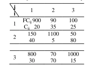
Table 5a. Transportation cost data (Cij & FCij).
Table 5b. Suppliers’ data (Pit, CUi, SHi & SIi0).
Table 5c. Customers’ data (Djt, CHj, BCj, BLj0 & CIj0).
j
∑Djt
1 2 3
Djt t
1 60 60 70 190 2 60 20 30 110 3 90 60 40 190 CHj 5 10 15 - BCj 20 40 30 - BLj0 0 20 0 - CIj0 0 0 30 -
5.4. GA and SAA based meta-heuristics solutions
The distribution schedule (Tables 6 and 7) and total production-distribution cost (Z) of the above example problem are given as follows (solved using GA and SAA separately).
Z (near opt) = 27,170.00 (GAs solution)
Z (near opt)= 27,790.00 (SAAs solution)
5.5. Equivalent variable cost solution
The equivalent variable cost matrix and the optimal distribution schedule (solved using LINGO solver) of the relaxed problem are given in Tables 8 and 9 respectively. The substitution of the optimal solution in Eqs. (1) and (11) respectively provides equivalent variable cost solution Z(EVC) and lower bound
value Z(L).
Z (L) = 27,170.00 (Lower bound value) Z (EVC) = 28,510.00 (Equivalent variable cost solution)
6. Computational results and performance analysis
To evaluate the performance of the proposed heuristics, computational experiments were done on 40 test problems. Forty test problems along with their outputs are considered for this performance comparison. The comparisons reveal the followings: Equivalent variable cost method provides only approximate solutions to all the test problems but very few of them are close or equal to GA and SAA solutions. EVC heuristic can also provide the lower bound value of the problem; GA and SAA based heuristics generate better solutions than the EVC heuristic and are capable of providing solutions close or equal to lower bound values. The average percentage deviation of GA based heuristic with lower bound value is 2.12%. The average percentage deviation of SAA based heuristic with lower bound value is 2.21%. The average percentage deviation of EVC heuristic with lower bound value is 8.89%. They are depicted in Fig. 1.
j
i 1 2 3
1 FCij 900 Cij 20
90 35
100 25
2 150 40
1100 5
50 80
3 800 30
70 70
1000 15
i
∑Pi t 1 2 3
Pit t
1 60 40 60 160 2 50 30 60 140 3 80 60 30 170
SHi 15 12 28 -
SIi0 10 0 0 -
Table 6. Distribution schedule using GA.
t
1 2 3
j
i 1 2 3
SIi1
1 2 3
SIi2
1 2 3
SIi
3
1 30 40 0 40 10 90 0
2 40 0 30 0 60 0
3 60 0 60 0 30 0
BLj
t
0 10 0 0 0 0 0 0 0
CIit
0 0 0 0 0 10 0 0 0
Table 7. Distribution schedule using SAA.
t
1 2 3
j
i 1 2 3 SIi1 1 2 3 SIi2 1 2 3 SIi3
1 40 30 0 40 10 80 10 0
2 40 0 20 10 10 60 0
3 60 0 60 0 30 0
BLjt 0 0 10 0 0 0 0 0 0
CIit 0 0 0 0 0 0 0 0 0
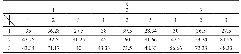
Table 8. Equivalent variable cost (EVCijt) matrix.
t
1 2 3
j
i 1 2 3 1 2 3 1 2 3
1 35 36.28 27.5 38 39.5 28.34 30 36.5 27.5
2 43.75 32.5 81.25 45 60 81.66 42.5 23.34 81.25
3 43.34 71.17 40 43.33 73.5 48.33 56.66 72.33 48.33
Table 9. Optimal distribution schedule for the relaxed problem.
t
1 2 3
j
i 1 2 3 SIi1 1 2 3 SIi2 1 2 3 SIi3
1 40 30 0 20 30 0 70 10 0
2 40 0 10 20 20 60 0
3 50 10 0 60 0 30 0
BLjt 10 0 0 0 0 0 0 0 0
7. Conclusions
This paper proposes GA and SAA based meta-heuristics and EVC based simple meta-heuristics to solve the MPFCPDP problem. The proposed methodologies are evaluated by comparing their solutions with lower bound values. The comparison of results reveal that the GA and SAA generate better solutions than the EVC solutions and are capable of providing solutions close or equal to the lower bound values. This paper concentrates on single-stage multi-period fixed charge model. As a future research, the single period formulation to the proposed multi-period fixed charge problem facilitates its scope for extending this to multi-stage supply chain problems.
References
[1] C. D. Flippo and G. Finke, “An integrated model for an industrial production- distribution problem,” IIE Transactions, Vol. 33, pp. 705-715, (2001).
[2] P. Chandra, and M. L. Fisher., “Coordination of production and transportation planning,” European Journal of Operational Research, Vol. 72, pp. 503-517,(1994).
[3] N. Rizk, A. Martel, S. D. Amours, “Synchronized production–transportation planning in a Single-plant multi-destination network,” Journal of the Operational Research Society, Vol.59, pp.90-104, (2008).
[4] D. Kim, P. M. Pardalos, “ A solution approach to the fixed charge network flow problem using a dynamic slope scaling procedure,” Operations Research Letter, Vol. 24, pp. 195-203 ,(1999). [5] N. Haq, Prem Vrat, and Arun Kanda,
“An integrated production-distribution model for manufacture of urea: a case,” International Journal of Production Economics, Vol. 39, pp. 39-49, (1991). [6] G. Barbarosogluand and D. Ozgur,
“Hierarchical design of an integrated production and 2-echelon transportation system,” European Journal of Operational Research, Vol. 118, pp. 464- 484, (1999).
[7] J. U. Kim, and Y. D. Kim, “A Lagrangian relaxation approach to multi-period inventory/distribution planning,” Journal of the Operational Research Society, Vol.51, pp. 364-370, (2000). [8] P. Kaminsky and D. Simchi-Levi,
“Production and transportation lot sizing in a two stage supply chain,” IIE
Transactions, Vol.35, pp. 1065-1075, (2003).
[9] Y. B. Park, “An integrated approach for production and distribution planning in supply chain management,” International Journal of Production Research, Vol. 43(6), pp. 1205-1224, (2005).
[10] T. F. Abdelmaguid and M. M. Dessouky, “A Genetic algorithm approach to the integrated inventory-distribution problem,” International Journal of Production Research, Vol. 44 (21), pp. 4455-4464, (2006).
[11] F. Z. Sargut and H. E. Romeijn, “Capacitated production and subcontracting in a serial supply chain,” IIE Transactions, Vol. 39, pp. 1031-1043, (2007).
[12] A. S. Safaei, S. M. Moattar Husseini, R. Z. Farahani, F. Jolai and S. H. Ghodsypour, “Integrated multi-site production-distribution planning in supply chain by hybrid modeling,” International Journal of Production Research, Vol.48 (14), pp. 4043-4069, (2010).
[13] D. E. Goldberg, “Genetic algorithms in search, Optimization and Machine Leaning,” Addison Wesley Limited: U.S.A, (2000).
[14] M. Gen, A. Kumar, J. R. Kim, “Recent network design techniques using evolutionary algorithms,” International Journal of Production Economics, Vol. 98, pp. 251-261.
[15] W. Dullaert, M. Sevaux, K. Sorensen, “Applications of Meta-heuristics,” European Journal of Operational Research, Vol. 179, pp. 601- 604, (2007). [16] S. Parthasarathy and C. Rajendran, , “An
experimental evaluation of heuristics for scheduling in a real life flow shop with sequence-dependent set up time of jobs,” International Journal of Production Economics, Vol. 49, pp. 255-263 ,(1997). [17] S.G. Ponnambalam, N. Jawahar, and P. Aravindan, “A Simulated Annealing Algorithm for Job Shop Scheduling,” Production Planning and Control, Vol.10, pp. 767-777, (1999).
[18] V. Jayaraman and A. Ross, “A simulated annealing methodology to transportation network design and management,” European Journal of Operational Research, Vol.144, pp 629-645, (2003). [19] B. Suman and P. Kumar ,A survey of
simulated annealing as a tool for single and multi-objective optimization,” Journal of Operational Research Society, Vol. 57, pp. 1143-1160, (2006).
[20] A. N. Balaji and N. Jawahar, “A Simulated Annealing Algorithm for a two-stage fixed charge distribution problem of a Supply Chain,” International Journal of Operational Research, Vol. 7(2), pp. 192-215, (2010). [21] S. A. Mansouri, “A simulated annealing
approach to a bi-criteria sequencing problem in a two-stage supply chain,” Computers & Industrial Engineering, Vol.50, pp. 105-119, (2006).