Information Theoretic Models for Dependence Analysis And missing Data Estimation

(1)

Published online March 10, 2013 (http://www.sciencepublishinggroup.com/j/ajtas) doi: 10.11648/j. ajtas.20130202.12

Information theoretic models for dependence analysis

and missing data estimation

D. S. Hooda, Permil Kumar

Department of Mathematics, Jaypee University of Engineering andTechnology, A.B. Road, Raghogarh, Distt.Guna-473226 (M.P.) India Department of Statistics, University of Jammu, Jammu-(India)

Email address:

ds_hooda@rediffmail.com (D. S. Hooda), Parmil@yahoo.com (P. Kumar)

To cite this article:

D.S.Hooda, Permil Kumar. Information Theoretic Models for Dependence Analysis And missing Data Estimation, American Journal of Theoretical and Applied Statistics. Vol. 2, No. 2, 2013, pp. 15-20. doi: 10.11648/j.ajtas.20130202.12

Abstract:

In the present communication information theoretic dependence measure has been defined using maximum

entropy principle, which measures amount of dependence among the attributes in a contingency table. A relation between information theoretic measure of dependence and Chi-square statistic has been discussed. A generalization of this informa-tion theoretic dependence measure has been also studied. In the end Yate’s method and maximum entropy estimainforma-tion of missing data in design of experiment have been described and illustrated by considering practical problems with empirical data.

Keywords:

Maximum Entropy Principle, Contingency Table, Chi-Square Statistics, Lagrange’s Multipliers And

Depen-dence Measure

1. Introduction

The frequencies of data based on counting of objects or units are categorized in a classified table known as contin-gency table. It can be defined as a rectangular array of order (m×n) having mn cells, where m and n are the number of rows and columns, which are equal to the number of cate-gories of two attributes.In matrix notation, we have the fol-lowing Contingency Table:

Table

Attribute B Total

B₁ B2 Bi Bn

A1 O11 O12 O2i O1n r1

A2 O21 O22 O2i O2n r2

Bi Oi1 Oi2 Oii Oin ri

Bm Om1 Om2 Omi Omn rm

total c1 c2 ci cn T

In above table, Oij, the (i,j)th cell represents the frequen-cy of characteristics of Ai and Bj, and ri and cj are the mar-ginal row and column sum totals.

The null hypothesis H0 of independence of attributes against H1 that attributes are dependent can be tested by

chi-square test statistic i.e.

∑∑

(

)

= =

−

=

m

i n

j _ij

ij ij

e

o

1 1

2 2

χ

(1)

where e_ij is the expected frequency corresponding to

(i,j)th cell having observed frequency O_ij. Under the null

hypothesis of independence

eij =

T

c

r

_i _j

where

T =

∑

=

m

i 1

ri =

∑

=

n

j 1

cj (2)

A decision about H₀ is made by comparing the value of

calculated chi-square i.e. (1) with the tabulated value of

chi-square for (m-1) (n-1) degrees of freedom at α % level

of significance.

In section 2, an information theoretic dependence meas-ure has been derived by using maximum entropy principle, which measures amount of dependence among the

(2)

and χ2 statistic has been discussed in section 3. In section 4, a generalized information theoretic dependence measure has been studied. Yate’s method and maximum entropy estimation of missing data in design of experiments have been described in section 5.

2. Information Theoretic Dependence

Measure

Contingency table paves the way for the analysis of cate-gorical data in physical and social sciences. But, many times only row and column totals are provided. In such cases we make use of Maximum Entropy Principle (MEP) which gives the same estimate as given by the hypothesis of independence. Soofi and Gokhale (1997) presented an in-formation theoretic formulation, which gave an insight into the degree of dependence among the factors of contingency

table. Let O_ij be the observed frequency in ith row and jth

column of the m × n contingency table. Let r₁, r₂,...,r_m

and c₁, c₂,...,c_n be the row and column sums or row and

column marginal totals such that

∑

=

n

j1

Oij = ri, i = 1,2,...,m (3)

∑

=

m

i1

Oij = cj, j = 1,2,...,n (4)

And

∑ ∑

= =

m

i n

j

1 1

Oij =

∑

=

m

i1

ri =

∑

=

n

j1

cj = T (5)

In case only the marginal totals information is provided to us, then the cell frequencies have to be estimated. We can fill only(m-1)(n-1)cell frequencies arbitrarily and determine the mn-(m-1)(n-1) = m + n-1 cell frequencies subject to (3), (4) and (5). Thus, there can be infinite number of sets that will be consistent with the given row and column totals. Out of these, we choose one which has maximum entropy as the above described situation demands the use of MEP i.e. we should choose the cell values so as to maximize

S = -

∑ ∑

= =

m

i n

j

1 1 T

x_ij log

T

x

_ij

(6)

Subject to

∑

=

n

j1

xij = ri, i = 1,2,...m (7)

∑

=

m

i1

xij = cj, j = 1,2,...n (8)

And

∑ ∑

= =

m

i n

j

1 1 xij = T (9)

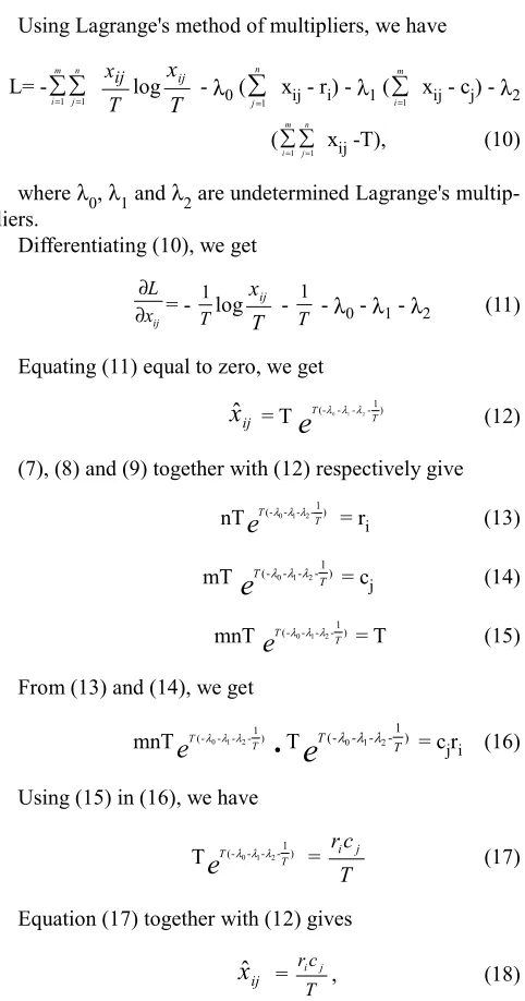
Using Lagrange's method of multipliers, we have

L= -

∑ ∑

= =

m

i n

j

1 1 _T

x_ij log

T x_ij

- λ₀ (

∑

=

n

j1

x_ij - r_i) - λ₁ (

∑

=

m

i1

x_ij - c_j) - λ₂

(∑ ∑

= = m

i n

j

1 1 xij -T), (10)

where λ₀, λ₁ and λ₂ are undetermined Lagrange's

multip-liers.

Differentiating (10), we get

ij

x L ∂

∂

= -

T 1

log

T xij

-

T 1

- λ₀ - λ₁ - λ₂ (11)

Equating (11) equal to zero, we get

ij

x

jri (16)

Using (15) in (16), we have

T

_e

T T)

1

-(λ0λ1λ2 = T

c ri j

(17)

Equation (17) together with (12) gives

ij

x

ˆ

= T

c ri j

, (18)

which is the maximum entropy estimate of the (I,j)th cell frequency.Let us denote this maximum entropy estimate by

e_ij. Then, maximum entropy is

S_max= -

∑ ∑

T xˆ_ij

log

T xˆ_ij

= -

∑∑

T eij

log T e_ij

= -

∑ ∑

₂

T c r_i _j

log ₂

T c r_i _j

= -

∑

i _T

r_i log

T r_i

-

∑

_j

T c_j

log T c_j

= S_r+ S_C , (19)

(3)

to-tals respectively.

Let O_ij's be the observed cell frequencies, then the

entro-py is given by

S = -

∑ ∑

_i _j O_Tij

log

T Oij

(20)

Since S_max≥ S, therefore,

S_r + S_C≥ S

It implies

D = S_r + S_C- S ≥ 0, (21)

where D is the difference between S_max and S and is

called information theoretic measure of dependence [refer to Watanabe (1969) and Kapur and Kesavan (1992)].

Actually, D > 0, measures the information contained in contingency table in addition to information given by row and column sum totals.

From (21), we know

D = - ∑i

T ri

log

T ri

-

∑

_j

T c_j

log T cj

+

∑ ∑

i j

T O_ij

log T O_ij

= -

∑ ∑

i j

T Oij

log T r_i

T cj

+ ∑ ∑i j

T

O

ij

log T Oij

= ∑ ∑i j

T Oij

log

ij ij

e O

(22)

It vanishes if and only if

T Oij

= T r_i

T cj

Or

O_ij = T

c ri j

= e_ij

Thus, we can conclude that the maximum entropy

esti-mates e_ijare equal to the estimates obtained from the

hypo-thesis of independence. The amount of deficit or difference

between O_ij and e_ij values is due to the association or

de-pendence between the factors of contingency tables. So, D is an information theoretic measure, which can be used for measuring the dependence between the factors of contin-gency table.

3. Information Theoretic Dependence

Measure and

χχχχ

2

In this section we study the relationship between

infor-mation theoretic dependence measure D and χ2 statistic.

Let

O_ij = e_ij + ∈_ij (23)

where ∈_ij is very small quantity,

Since

∑ ∑ = = m i

n j

1 1 Oij =

∑ ∑

₌ ₌

m

i n

j

1 1 eij = T (24)

And

∑ ∑

= =

m

i n

j

1 1

O_ij =

∑∑

= =

m

i n

j

1 1

e_ij +

∑ ∑

= =

m

i n

j 1 1 ∈ij

therefore

∑ ∑

= =

m

i n

j

1 1

∈ij = 0 (25)

(22) together with (23) gives

D =

∑ ∑

= =

m

i n

j

1 1 T

eij+εij log (

ij ij ij

e e +ε

)

=

∑ ∑

= =

m

i n

j

1 1 T

eij+εij

log (1+

ij ij

e

ε

)

=

∑ ∑

= =

m

i n

j

1 1 T

eij+εij [

ij ij

e

ε

-2 1

2 2

ij ij

e ε

+ 3

3

3 1

ij ij

e ε

+...]

=

∑ ∑

= =

m

i n

j

1 1 _T

ij ε

+

∑ ∑

= =

m

i n

j 1 1 2T

1

ij ij

e

2

ε

+ ...

Using (25) and neglecting higher order terms, we have

D ~

∑ ∑

= =

m

i n

j

1 1 2T

1

ij ij e

2

ε

=

T

2 1

_{∑ ∑}

= =

m

i n

j

1 1 ij ij ij

e e O - )2 (

=

T

2 1

2 (26)

Thus, D gives times chi-square information or χ2 gives

2T times the additional information given by the observed frequencies over the information already provided by the

row and column totals. It is worth mentioning that χ2 test

does not give us the degree of dependence, while it is pro-vided by information theoretic measure of dependence D.

Moreover, χ2 statistic cannot be used for comparing the

several tables. Many coefficients have been proposed to measure the association between row and column factors, viz., Yule's coefficient Q of association, Pearson's

coeffi-cients φ2 of mean square contingency, etc.

(4)

normalized D is given by

D_N = e-D

For D = 0, D_N takes value one and for very large D, D_N

is 0. It implies 0 ≤ D_N≤ 1. It may be noted that when D_N

=1, attributes or factors are independent and for D_N = 0,

factors are perfectly dependent.

4. Generalized Measure of Dependence

In the present section, we study a generalized measure of dependence in contingency table of which D given by (2.19) is a particular case.

We choose the cell frequency which maximizes Harvda

and Charvat (1967) entropy of degree β given below:

m n

ij

i 1 j 1

x 1

S 1 , ( 0) 1

1 T

β β

= =

 _ _ 

 

= _   − _ β > ≠

− β_

∑∑

  _ (27)

subject to

∑

=

n

j 1

x_ij = r_i (28)

∑

=

m

i1

x_ij = c_j (29)

and

∑ ∑

= =

m

i n

j

1 1

x_ij = T (30)

We use Lagrange's method of multipliers to maximize (27) subject to constraints (28) to (30).

L = _β

-1

1

[ ( )β

T x_ij

-1]+ λ₀ (

∑

=

n

j 1

x_ij - r_i)

+ λ₁ (

∑

=

m

i1

x_ij - c_j) + λ₂ (

∑ ∑

= =

m

i n

j

1 1

x_ij - T), (31)

where λ₀, λ₁ and λ₂ are undetermined Lagrange's

multip-liers. Now, differentiating (31) w.r.t. x_ij and equating it to

zero, we get

ij

x L ∂

∂

=₁_-1_β[ -1

. .

1 _β

β βxij

T + λ0 + λ1 + λ2 ] = 0

It implies

β β

-1 β

β

T

1 -ij

x

= - λ₀ - λ₁ - λ₂

1

-β

ij

x

= β_β-1 Tβ (λ₀ + λ₁ + λ₂)

Or

ij

x

ˆ

= [β_β-1 Tβ (λ₀ + λ₁ + λ₂) ]

1 -1

β (32)

where λ₀, λ₁ and λ₂ to be determined using (28), (29)

and (30). Equations (28), (29) and (30) together with (32) respectively give

n [β_β-1 Tβ (λ₀ + λ₁ + λ₂) ]

1 -1

β = ri (33)

m [β_β-1 Tβ (λ₀ + λ₁ + λ₂) ]

1 -1

β = cj (34)

and

mn [β_β-1Tβ (λ₀ + λ₁ + λ₂)] ]

1 -1

β = T (35)

From (33) and (34), we have

mn [β_β-1Tβ(λ₀+λ₁+λ₂) ]

1 -1

β [ _β

β-1

Tβ(λ₀+λ₁+λ₂) ]

1 -1 β

= r_ic_j (36)

From (36) and (35) we get

[β_β-1Tβ (λ₀ + λ₁ + λ₂)]

1 -1

β = _T

c r_i _j

(37)

On putting the value of (37) in (32), we have

ij

x

ˆ

= T

c r_i _j

(38)

Thus, (38) is the maximum entropy estimate of the (i, j)th

cell frequency denoted by e_ij.Hence

max

β

S

= _β

-1

1

[

∑ ∑

= =

m

i n

j 1 1

( T eij

)β -1]

=

β -1

1

[

∑ ∑

= =

m

i n

j

1 1

(

1

[

∑

=

m

i 1

(

T

ri _{) -1] (40)}

is

β

degree entropy of row total and

β

c

S

= _β

-1

1

[

∑

=

n

j 1

(

T

_rβ Scβ (42)

Since

S

βmax ≥ Sβ, therefore,

β

cβ - S

β _≥_{0, (43)}

which is equal to 0 if

max

β

S = Sβ. Thus, Dβ is generalized

information theoretic dependence measure between the factors of contingency tables and reduce to D given by (21)

in case _β_→₁.

5. Estimation of Missing Data in Design

of Experiments

In field experiments we design the field plots. In case we find one or more observations missing due to natural ca-lamity or destroyed by a pest or eaten by animals, it is cumbersome to estimate the missing value or values as in field trials it is practically impossible to repeat the experi-ment under identical conditions. So we have no option ex-cept to make best use of the data available. Yates (1933) suggested a method:

“Substitute

x

for the missing value and then choose

x

so as to minimize the error sum of squares”.

Actually, the substituted value does not recover the best information, however, it gives the best estimate according to a criterion based on the least square method.

For the randomized block experiment

(

−1

)(

−1

)

− + =

q p

T qQ pP

x ₍₄₄₎

where

=

p

Number of treatments,

=

q

Number of blocks

=

P

Total of all plots receiving the same treatment as

the missing plot

=

Q

Total of all plots in the same block as the missing

plot

=

T Total of all plots

For the Latin Square Design, the corresponding formula is

(

)

(

1

)(

1

)

2

− −

− + + =

q p

T P P P p

x r c t

(45)

where

=

Grand total

In case more than one plot yields are missing, we substi-tute the average yield

...,

are known

yields and

x

is the missing yield. We obtain the

maxi-mum entropy estimate

for

x

by maximizing:

∑

= + + − + +

− n i

i i

x T

x x T

x

0

log

log (46)

Thus we get

[

...

]

,

ˆ

1

2 1

2

1 x _T

n x x

_x

n

x

=

(47)

where

∑

= = n

i i

x T

1

and the value given by (47) is called

maximum entropy mean of

x

₁

,

x

₂

,

...,

x

_n.

]

, ...

1 2 2 1

1 n T y

x n x x

x x

x +

= (48)

y

ˆ

[

2_...

]

1 _, 2

1

1 T x

n x n x x

x x

x +

= (49)

The solution of (48) and (49) is

[

xn

]

T

n x x

x

y

x

1 2 2 1 1

...

ˆ

=

(50)

Hence all the missing values have the same estimate and this does not change if the missing values are estimated one by one.

There are three following drawbacks of the estimate giv-en by (47)

(i)

_x

⌢

_{is rather unnatural. In fact}

_x

⌢

_{is always greater than}

Arithmetic mean of

x

₁

,

x

₂

,

...,

x

_n.

(ii) If two values are missing, the maximum entropy es-timated for each is the same as given by (50).

(iii) This is not very useful for estimating missing values in design of experiments.

(6)

use Burg’s [1] measure given by

B (P) =

∑

=

n

i i

p

1

log (51)

Then we get the estimate

x

⌢

₌

n x x

x₁ + ₂... + _n

=

x

(52)

In fact we choose a value

_x

⌢

_{, which is as equal to}

n

x

₁

,

₂

,

...,

as possible and so we maximize a measure of

equality. Since there are many measures of equality, there-fore our estimate will also depend on the measure of equali-ty we choose.

The second drawback can be understood by considering the fact that the information theoretic estimate for a missing value depends on:

(a) The information available to us

(b) The purpose for which missing value is to be used. The third drawback, as according to the principle of max-imum entropy, we should use all the information given to us and avoid scrupulously using any information not given to us. But in design of experiments, we are given informa-tion about the structure of the design which we are not us-ing this knowledge in estimatus-ing the missus-ing values. Con-sequently, the estimate is not accurate, however, method defined in section 2 be applied to estimate the missing

val-ue

x

ij in contingency tables. Accordingly, the value

x

ij is to

be chosen to minimize the measure of dependence D.

References

[1] Burg J.P.(1970). “The relationship between Maximum En-tropy Spectra and Maximum Likelihood in Modern Spectra Analysis”, ed D.G. Childers, pp130-131.

[2] Harvda, J. and Charvat, F. (1967). Quantification method of classification processes concepts of structural - entropy, Kybernetika, 3: 30-35.

[3] Kapur, J.N. and Kesavan, H.K. (1992).” Entropy optimiza-tion principles with applicaoptimiza-tions.” Academic press, San Di-ego.K. Elissa, “Title of paper if known,” unpublished.

[4] Soofi, E.S. and Gokhale, D.V. (1997). “Information theoretic methods for categorical data. Advances in Econometrics.”, JAI Press, Greenwich.

[5] Watanabe,S.(1969).”Knowing and Guessing”.John Wi-ley,New York,1969.

[6] Watanabe, S. (1981). “Pattern recognition as a quest for minimum entropy.”, Pattern Recognition. 13:381-387.