IIIInternational
nternational
nternational
nternational JJJJournal of
ournal of
ournal of
ournal of
Agriculture and Biosciences
Agriculture and Biosciences
Agriculture and Biosciences
Agriculture and Biosciences
www.ijagbio.com; editor@ijagbio.com
Research Article
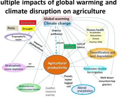
Impacts of Climate Change on Agricultural Systems
Abolfazl Davari
Higher Educational Complex of Saravan
*Corresponding author: abolfazl.davari23@gmail.com
Article History: Received: February 25, 2016 Revised: May 28, 2016 Accepted: June 26, 2016
A B S T R A C T
Describing climate change by the increase in average temperatures is inescapably useful, but at the same time often misleading. Increases in global average temperature of only a few degrees, comparable to normal month-to-month changes in many parts of the world, will have drastic and disruptive effects. Agriculture has always been dependent on the variability of the climate for the growing season and the state of the land at the start of the growing season. The key for adaptation for crop production to climate change is the predictability of the conditions. What is required is an understanding of the effect on the changing climate on land, water and temperature. Research on crop yields has received significant attention on a variety of scientific fronts. Plant and soil science research has provided an indication of the potential of the Canadian prairies to produce food and fibre with given conditions. Across the prairies, crops yields will vary. All crops in Manitoba may decrease by 1%, Alberta wheat, barley and canola may decrease by 7% and Saskatchewan wheat, barley and canola may increase by 2-8%.
Key words: Yields, Temperature,Livestock, Water, Sustainability
INTRODUCTION
The Current State of Knowledge
Early research on agricultural impacts led to some rather dire predictions of adverse impacts of climate change on food production, and the public perception that climate change may lead to global food shortages continues today. Although state-of-the-art at the time, the early predictions involved relatively simple data and methods, typically estimating the effects of increases in average annual temperature on yields of a limited number of crops at a limited number of locations, and extrapolating the typically negative effects to large regions. With advances in data and models, most assessments of the impacts of climate change on agriculture predict that the world’s ability to feed itself is not threatened by climate change. The most recent IPCC report on Impacts and Adaptation finds that climate change is likely to have both positive and negative impacts on agriculture, depending on the region and the type of agriculture. Overall, the report predicts that during the present century there will be a “marginal increase in the number of people at risk of hunger due to climate change.” (Easterling et al., 2007). However, research also shows that this finding should not lead to complacency, as analysis also suggests that some of the poorest and most
vulnerable regions of the world are likely to be impacted negatively, and in some cases, severely. One of the most important advances made in response to these early studies was to recognize that economic agents in this case, farmers and the various private and public institutions that support agriculture – would adapt to climate changes in ways that would tend to mitigate negative impacts and take advantage of positive impacts. Another important advance in research was to recognize that there would be substantially different local, regional and global impacts. As data and modeling capability has improved, it has become increasingly clear that there are likely to be substantial adverse changes in some particularly vulnerable regions, such as in the semi-arid tropics, but there is also likely to be positive changes in the highland tropics and in temperate regions (Parry et al., 2004).This article is review and the aims are climate change impacts on agricultural systems.
Crop Yields
Agriculture has always been dependent on the variability of the climate for the growing season and the state of the land at the start of the growing season. The key for adaptation for crop production to climate change is the predictability of the conditions. What is required is an understanding of the effect on the changing climate on
Fig 1: Projected impact of climate change on agricultural yields by the 2080s, compared to 2003 levels (Cline, 2007).
land, water and temperature. Research on crop yields has received significant attention on a variety of scientific fronts. Plant and soil science research has provided an indication of the potential of the Canadian prairies to produce food and fibre with given conditions. In reality, it is difficult to accurately predict crop yields, because of the variability of conditions and subsequently production on the prairies. An example of this is CO2 enrichment. Laboratory experiments have concluded the CO2 enrichment may benefit C3 crops (e.g. rice, wheat, soybeans, potatoes and vegetables), although these improvements found in laboratory experiments may not be realised in the field. A temperature rise extends the growing season and the farmable area, it causes earlier maturity of grain and opens up for the growing/farming of new crops. While the temperature rise is beneficial to the crops, the extra heat also affects weeds. Weeds, pests, and insects tend to get better living conditions under higher temperatures. To further increase the risks of a good crop, there is also the potential for poor herbicide performance. The combination of the weeds, pests and poor herbicide performance reduces the potential crop yields. The increase in temperature also increases evaportranspiration, which has a negative impact on crop yields. During the growth cycle of the plant, water is needed at the initial stages of production, but not during the final stages. Low levels of precipitation have a negative effect on the germination of the seeds. Dry conditions, frequency and severity of dust storms all result in decreased production of major grains. Given the potential changes in production variables, it is estimated that the average potential yields may fall by 10-30% (Williams et al., 1988). Across the prairies, crops yields will vary. All crops in Manitoba may decrease by 1%, Alberta wheat, barley and canola may decrease by 7% and Saskatchewan wheat, barley and canola may increase by 2-8% (Arthur, 1988).
Temperature thresholds for crop yields
Describing climate change by the increase in average temperatures is inescapably useful, but at the same time often misleading. Increases in global average temperature of only a few degrees, comparable to normal month-to-month changes in many parts of the world, will have drastic and disruptive effects. A recent study suggests that it may be easier for people to perceive climate change as reflected in temperature extremes, such as the marked increase in the frequency of temperatures more than three standard deviations above the local summer norm for 1951-80 (Hansen et al. 2012).
An important new wave of research shows that crops, too, are often more sensitive to temperature extremes than to averages. In many cases, yields rise gradually up to a temperature threshold, then collapse rapidly as temperatures increase above the threshold. This threshold model often fits the empirical data better than the earlier models of temperature effects on yields. It is obvious that most crops have an optimum temperature, at which their yields per hectare are greater than at either higher or lower temperatures. A simple and widely used model of this effect assumes that yields are a quadratic function of average temperatures.8 The quadratic model, however, imposes symmetry and gradualism on the temperature-yield relationship: temperature-yields rise smoothly on the way up to
have grown these crops for many years, without any evidence of a large-scale shift to more heat-resistant crops or cultivars; temperature-yield relationships are quite similar in northern and southern states (Schlenker and Roberts, 2009). Thus adaptation is an important possibility, but far from automatic.
Livestock production
The main effects of climate change on livestock from increased temperature and decreased precipitation is distress, but because livestock do not have the same limitations as crops there are potential benefits to expanding acreage. The increasing temperatures can have varying effects, depending on when they occur. Warmer conditions in the summer can lead to stress on range and housed livestock since dry pastures, poor hay and feed production and shortages of water all lead to worse conditions for cattle (Arthur, 1988).On the other hand, increased temperatures during the winter months can reduce the cold stress experienced by livestock remaining outside, as well as reduce the energy requirements to heat the facilities of those banimals inside. In the previous section, it was mentioned that crops required class 3 or better land to produce acceptable yields, however, to produce acceptable pastures does not have the same restrictions. The increased temperature would have a positive effect on the growth of the pasture, and provide better feed for livestock. This assumes that the pastures are in areas where moisture is not a critical issue. Water resources are critical to a successful livestock operation. All livestock operations require good quality drinking water, and without it livestock will not survive. As with crops, diseases and insects could have an adverse effect on much of the livestock industry. Insects and diseases that livestock is unaccustomed to could move into the production area. Secondary effects such as dust storms and wind erosion also factor into the worsening conditions for livestock. Livestock is more resistant to climate change than crops because of its mobility and access to feed. Livestock production could be one of the key methods for farmers to adapt to climate change through diversification of their farming mix (Arthur, 1988).
Climate change, water and agriculture
Warming is increasing the atmosphere’s capacity to hold water, resulting in increases in extreme precipitation events (Min et al., 2011). Both observational data and modeling projections show that with climate change, wet regions will generally (but not universally) become wetter, and dry regions will become drier (Sanderson et al. 2011; John et al. 2009). Perceptible changes in annual precipitation are likely to appear in many areas within this century. While different climate models disagree about some parts of the world, there is general agreement that boreal (far-northern) areas will become wetter, and the Mediterranean will become drier (Mahlstein et al., 2012). With 2°C of warming, dry-season precipitation is expected to decrease by 20 percent in northern Africa, southern Europe, and western Australia, and by 10 percent in the southwestern United States and Mexico, eastern South America, and northern Africa by 2100 (Giorgi and Bi, 2009).10 In the Sahel area of Africa, the timing of
Agriculture policy
Government policies have had a significant impact on current agriculture and will continue to do so (Tyrchniewicz and Wilson, 1994). Previous agriculture policies, such as the Western Grain Transportation Act and the Canadian Wheat Board Act, rewarded expansion of cropland and made land-use changes difficult (Baydack et. al., 1996). Many policies of the past have not considered the need for adaptation, because it was not viewed as an issue. Some of the current income protection policies such as crop insurance, and the Gross Revenue Income Program, need to be reviewed with adaptation as a guiding force. Many of these programs and policies encourage certain farming techniques and products and can have a major effect on adaptation. For example, if farmers have a guaranteed income when they use a certain practice (which may or may not be sustainable) then they will be encouraged not to use another practice which could be sustainable since it is not insurable and thus does not have a guaranteed income. As a result, many farmers make products that are insurable, using techniques that are insurable despite the sustainability, or in this case, climate change implications. The current shifts in agriculture policy are starting to allow more flexibility in production, not only in techniques, but also in products. Agriculture and Agri-food Canada has introduced a program called the Canadian Adaptation and Rural Development Fund. The focus of this program has been to assist rural communities and farmers in adapting to changes in economic policies. While the program is not aimed at climate change, there is potential to use it to have agriculture adapt to more than just economic policies. At the moment, however, the issue of climate change is viewed only from the mitigation perspective, in terms of agriculture's capacity to reduce greenhouse gas emissions and act as a carbon sink. The issue of impacts and adaptation is grossly neglected within the debate involving climate change and sustainable agriculture (Agriculture and Agri-food Canada, 1996). Unless there is a substantial shift in the thinking of Agriculture and Agri-food Canada regarding climate change and agriculture, the economic policies designed to help facilitate adaptation to changing global economic conditions may turn out to be a missed opportunity.
Agriculture and Sustainability
In terms of the effect of changing crop mixes and revenues on the rest of the prairie economies, other sectors will be affected by expenditures for farm inputs and consumer goods and services. Discretionary expenditures change in direct response to changes in cash flow, hence those scenarios that produce a negative effect on prairie agriculture will pass on those negative effects to other sectors too but to a lesser degree (Arthur, 1988). While it is tempting to compare results from different sources, this should be done with caution since these studies have all been done using different assumptions and methodologies. Furthermore, most studies only take the effect of climate change into account while all other factors are held constant. Given the complexity of combining climate change models with economic and other models and the degree of uncertainty inherent in all of these models, figures and predictions that are presented
deficits may preclude these new crops as an adaptation option. However, in order to adopt these new crops moisture deficits could be overcome through the use of irrigation (also an adaptive strategy). Decreasing availability of water for all users on the prairies will lead to conflicts as producers compete with recreationists, household users, electrical utilities, and the manufacturing and other industry for water for irrigation (Rosenberg, 1992; & Wittrock and Wheaton, 1992).
MATERIALS AND METHODS
This article is review and the aims of Climate change impacts on agricultural systems. The experiment 1 was conducted by Mary and Majule (2009). The study was carried out in Manyoni District in Singida Region, Tanzania. The district lies between 6°7°S and 34°35°E covering an area of 28,620 km2 that is about 58% of the entire area of Singida Region. Manyoni District was selected for the following reasons; first, it falls within the semi-arid areas of Tanzania where there are frequent food shortages due to uncertainty of rainfall. According to URT (2005) the 2000/01 household surveys, the district fell within regions with worst assessment of food poverty. In the district, 55% of its populations are living below the food poverty line. Average per capita earning of residents is estimated at 170 US dollars (URT, 2005). (Mary and Majule 2009). Second, the area provides an opportunity to study impacts associated with CC & V on crop and livestock and third it is within the project area on “Strengthening Local Agricultural Innovation Systems to adapt to climate change in Tanzania and Malawi Project”. The climate of Manyoni District is basically of an inland equatorial type modified by the effects of altitude and distance from the Equator. The district forms part of the semi-arid central zone of Tanzania experiencing low rainfall and short rainy seasons which are often erratic with fairly widespread drought of one year in four (Mary and Majule, 2009). Manyoni District has a unimodal rainfall regime, which is concentrated in a period of six months from November to April. The long-term mean annual rainfall is 624 mm with a standard deviation of 179 mm and a coefficient of variation of 28.7%. The long-term mean number of rainy days is 49 with a standard deviation of 15 days and a coefficient of variation of 30.6%. Generally rainfall in the District is low and unreliable. The annual mean, maximum and minimum monthly mean daily relative humidity is 80.6%, 86.0% (February) and 73.4% (July) respectively (Lema, 2008). The maximum and minimum monthly mean daily pan evaporation is 6.6 mm/day (November) and 5.2 mm /day (January) with standard deviations of 1.2 mm/day and 0.8 mm/ day respectively (Mary and Majule 2009). Temperatures vary according to altitude. The annual mean, maximum and minimum monthly mean daily temperatures in the District are 22.0°C, 24.4°C (November) and 19.3°C (July) respectively. The average annual daily sunshine hours are 7.9 h/day. The maximum and minimum monthly mean daily sunshine hours are 9.2 h/day (September) and 6.5 h/day (January) respectively. Both secondary and primary data were collected in order to address the objectives of this study. Secondary sources included published research papers and relevant reports,
rainfall and temperature data kept at Meteorological department, internet search and other relevant sources. Primary data were collected using multiple approaches including both quantitative and qualitative PRA methods were used to collect primary data from the study area. The methods used included key informant interviews, focus group discussion with at total number of 20 participants per village, household interviews to 10% of the total number of households per village, historical mapping of different climate related events over the past years that could be remembered, wealth ranking of different social economic groups based on local criteria they use and then direct field observations through transect walks. Qualitative data from various sources were examined and presented bin different forms. Quantitative were edited, coded and entered in a computer and the Statistical Package for Social Science (SPSS) software version 11.5 spread sheet was used for the analysis. Descriptive statistics were run to give frequencies and then cross-tabulation was undertaken. Multiple response questions were analyzed so as to give frequencies and percentages. Tables and bar charts were used to present different variables. Cross-tabulation allowed a comparison of different study parameters in the two villages. Temperature and rainfall data from meteorological stations were analyzed using Microsoft Office Excel 2003 to present patterns and trends of rainfall and temperature in the form of graphs (Mary and Majule, 2009).
simulations under the conditions that; there was no fertilizer deficiency and water stress (automated irrigation, 100% efficiency), 1st of October was planting date, and 250 seed m-2 sowing rate was used with 100% germination rate. Weeds, insects and crop diseases had no negative effect on yield. CERES-Wheat model was set to use Priestly-Taylor evapotranspiration model to calculate crop water requirement Weather data used in this study were generated using Autoregressive Moving-Average method (ARMA (p, q), with which daily average minimum and maximum data for each set of temperatures (0 and ±2, 4, and 6 0C, 0 represents long term average values of temperature and hereafter called as current) were simulated. Daily average solar radiation and precipitation values were average of 1975-2005 years (Tonkazi et al., 2010).
RESULTS AND DISCUSSION
In the experiment 1 was conducted by Mary and Majule (2009). Resource maps are important as it shows various resources available in the village in which peoples’ livelihood depend on. A village resource map Figure 2 in Kamenyanga village occupies 4480 hectares of land of which residential area is 920 ha, farm land is 1740 ha, grazing land 884 ha and 1016 ha is a village forest reserve area. Kintinku village covers an area of 3600 ha, 792 ha is residential areas, 1368 ha is farm land, 1436 ha is grazing land and 4 ha is village forest reserve area Figure 3. In terms of land resource (farmland) as well as forest cover, Kamenyanga village seems to be in a better position than Kintinku village and therefore communities are less vulnerable to impacts of CC & V. Their proportions of the groups were provided by the local people as presented in Table 1. Generally the stratification of the surveyed villages indicated that the poor group embodying the largest number of households (Mary and Majule, 2009). The percentage of rich category is low in both villages which implies that a high level of vulnerability of communities in these villages (Table 1). For comparison, the household numbers in the medium rich group in Kamenyanga were higher than those in Kintinku. Parallel to that, Kintinku led with the number of households in the poor group but also has a higher number of households falling in the rich group. Based on the characteristics of the three wealthy groups, it implies that vulnerabilities and adaptive capacities among groups vary accordingly in the two villages studied. Farming is the major economic activity for (61.8%) of the respondents in Kamenyanga and (56.9%) in Kintinku (Table 2). Although livestock is the second major economic activity in Kamenyanga (35.3%) and Kintinku (25.0%), all livestock keepers are also farmers and none of the respondents was keeping livestock alone. Petty business ranked as the third economic activity. However the activity appeared to be of less importance to Kamenyanga (2.9%) as compared to Kintinku (18.1%) (Mary and Majule, 2009).. This is due to the difference in the levels of urbanization in these two villages. Since Kintinku is more urbanized than Kamenyanga that means petty business opportunities are also higher. This implies that villagers in Kintinku stand a better chance of coping with the impacts of CC & V because they can diversify
economic activities more easily than villagers in Kamenyanga. Given that, farming and livestock keeping is the main economic activities in both villages this implies that CC & V will have a far-reaching effect on the livelihoods of these communities. Other minor economic activities included selling of local brew, which was common in Kamenyanga and was mainly done by women. According to interviews this activity has increased recently.In addition, currently there has been an increase in the number of women involved in the production of charcoal and the collection and selling of firewood. This is unlike in the past when these activities were only undertaken by men.
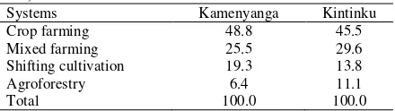
Also in Kamenyanga, there were few people involved in bee keeping. It was observed that most of these emerging activities are non-farm activities (Mary and Majule, 2009). However, the raw materials for preparing local brew depend on the availability of crops, whereas charcoal and firewood was harvested from the natural forest, which is also affected by the CC & V. Table 3 presents the existing farming systems in Kamenyanga and Kintinku villages, which include crop farming (referring to production of crops alone), mixed farming (referring to crop farming and livestock keeping), shifting cultivation and agroforestry. Figure 4 shows that (63.8%) of the respondents in Kamenyanga village and (73.8%) in Kintinku village perceived that there was an increase in temperature over the last 10 years.
It has been reported that over the last 10 years during September to December the area becomes extremely hot, especially in Kintinku and during the night it is very cold. Figure 5 show that, the majority of respondents (35.8%) and (36.2% perceived changes in onset of rains and decrease in precipitation (35.8%) and (24.5%) as well as increase in frequency of drought (24.7%) and (29.8%) in Kamenyanga and Kintinku respectively. The majority declared that rainfall onset has changed because they used to plant crops in October/November but nowadays they have to plant in December/January. Similar results were
Table 1: Distribution of Wealth Groups in Kamenyanga and Kintinku (Mary and Majule, 2009)
Village name
Total number of households
Rich group
Medium rich group
Poor group Kamenyanga 400 (100) 20 (5) 140 (35) 240 (60) Kintinku 411 (100) 41 (10) 62 (15) 308 (75)
Total 811 61 202 548
Table 2: Proportion (%) distribution of respondents’ main occupation (Mary and Majule, 2009)
Main occupation Kamenyanga Kintinku
Farming 61.8 56.9
Livestock keeping 35.3 25.0
Business 2.9 18.1
Total 100.0 100.0
Source: Field survey (2008).
Table 3: Farming systems by proportions (Mary and Majule, 2009)
Systems Kamenyanga Kintinku
Crop farming 48.8 45.5
Mixed farming 25.5 29.6
Shifting cultivation 19.3 13.8
Agroforestry 6.4 11.1
Table 4: Some of the selected soil properties used in the study FC, Field capacity; PWP, Permanent wilting point; BD, Bulk density, OM, Organic water (Tonkazi et al., 2010)
Depth, FC cm3 cm-3 PWP % BD, g cm-3 pH Sand Silt Clay Texture class
18 0.39 0.23 1.35 7.3 7.3 34.7 58 Clay
39 0.39 0.23 1.35 7.3 7.1 32.6 60.3 Clay
49 0.39 0.23 1.36 7.4 7.7 29.2 63.1 Clay
88 0.39 0.23 1.36 7.4 34.3 19.3 46.4 Clay
120 0.39 0.23 1.35 7.4 34.3 19.3 46.4 Clay
Table 5: CERES-Wheat model simulation results (Tonkazi et al., 2010)
Parameters CO2 levels (ppm)
Yield, kg ha-1 380 420 460 500
Lowest 5209 5312 5413 5498
Highest 10843 11101 11343 11579
Current 8287 8455 8611 8754
Average 8018 8183 8336 8478
% increase 37.14 37.17 37.14 37.19 % decrease 30.84 31.29 31.73 32.27 Flowering date (DAP)
Lowest 156 156 156 156
Highest 203 203 203 203
Current 181 181 181 181
Average 177 177 177 177
% increase 13.82 13.82 13.82 13.82 % decrease 12.16 12.16 12.16 12.16
reported whereby a significant number of farmers in eleven African countries believed that temperatures had increased and that precipitation had declined. Also reported the same. Local perceptions by farmers with respect to changes in temperature as well as increasing rainfall variability are closed related to empirical analysis of rainfall and temperature trends using the data obtained from meteorological station. Trend analysis of rainfall data indicated that annual rainfall decreased from 1922 to 2007, more pronounced decrease being from 1982 onwards.
Also shows that the onset of rainfall has shifted from October to November and that the rainy sea-son is shorter ending in March or April(Mary and Majule, 2009). What can be noted is that the area might be receiving the same amounts of rain but there are changes in distribution and therefore leading to floods and/or droughts (see for example a graph representing year 2000 – 2007).
Also the figure show there was changes in rainfall peak, see for example the graph representing year 1922-29 and 1930-39 compared to 1980-89 and 2000-07. For farmers, this implies increased risk of crop failure, due to poor seed germination, washing away of seeds and crops, stunted growth, drying of crops caused by changes in rainfall pattern and amount.
Sometimes this leads to re-ploughing and replanting thereby increasing production costs. For livestock, this implies decreased pasture and increased parasites and diseases due to decreased rainfall (drought) and increased (floods) rainfall (Mary and Majule, 2009). In the experiment 2 was conducted by Tonkazi et al. (2010). ARMA(3,1) and ARMA(3,2) models were well fitted to daily maximum and minimum temperatures series of the station, respectively. In order to generate synthetic data, residuals of the model fitted to certain probability distributions. Considering KS values, logistic and BetaGeneral distributions were found adequate for maximum and minimum temperatures series, respectively.
Synthetic temperature series were generated using the adequate models recombining periodic and probabilistic components of the series. At 380 ppm CO2 level, the lowest yield occurred at +6 0C, +6 0C treatment (max. and min. temperatures, respectively) as 5209 kg ha-1, while highest yield occurred as 10843 kg ha-1, at -60C,-60C treatment with an average yield of 8018 kg ha-1. At current temperatures (0 0C) and CO2 level (380 ppm) simulated yield was 8287 kg ha-1. Similarly, at 420 CO2 level, highest and lowest wheat yields were 11 101 and 5 312 kg ha-1, respectively (Table 6) (Tonkazi et al., 2010). Average and current yield at 420 ppm CO2 level were 8183 and 8455 kg ha-1, respectively. Likewise, highest and lowest wheat yields were simulated as 11343 and 5 413 kg ha-1 with current and average yields of 8611 and 8 336 kg ha-1 at 460 CO2 level, respectively (Table 6). In agreement with the other three levels, at 500 CO2 level maximum, minimum, current and average wheat yields turned out to be 11 579, 5 498, 8 754, and 8 478 kg ha-1, respectively. Also, when CO2 level was fixed, effect of both studied temperatures were similar and there was about 37% increase and 32% decrease in wheat yields compared to current situation (Table 3 and Figures 1 and 2). It was noticed that 4.5 0C increases in both temperatures would result in severe impact on wheat yield (Tonkazi et al., 2010).
REFERENCES
Ackerman F and C Munitz, 2012. Climate Damages in the FUND Model: The DSSAT cropping system model. 2003. Eur J Agron, 18: 235–265.
Ackerman F and EA Stanton, 2011. The Last Drop: Climate Change and the Southwest Water Crisis. Somerville, MA: Stockholm Environment Institute-US, 90: 329–347.
Ackerman F and EA Stanton, 2013. Climate Economics: The State of the Art. London: Routledge. Proceedings. Nat Acad Sci, 105: 5129–5133.
Agriculture and Agri-food Canada, 1996. Strategy for Environmentally Sustainable Agriculture and Agri-food Development in Canada. An entropy approach to spatial disaggregation of agricultural production. Agric Sys, 90: 329–347.
Auffhammer M, V Ramanathan and JR Vincent, 2011. “Climate change, the monsoon, and rice yield in India. Climatic Change J. 111: 411–24.
Barnett TP, JC Adam and DP Lettenmaier, 2005. “Potential impacts of a warming climate on water availability in snow-dominated regions Environment and Production Technology Division Discussion Paper. Nat Acad Sci, 438: 303–9.
scenarios in Haihe River, China. Theor Appl Climatol, 99: 149–61.
Easterling WE, PK Aggarwal, P Batima, KM Brander, L Erda, SM Howden, A Kirilenko, J Morton, J.-F. Soussana, J. Schmidhuber and FN Tubiello, 2007. Impacts, Adaptation and Vulnerability. Contribution of Working Group II to the Fourth Assessment Report of the Intergovernmental Panel on Climate Change, 12: 273-313.
Giorgi F and X Bi, 2009. Challenges to manage the risk of water scarcity and climate change in Mediterranean. Water Resoures Manag, 21: 227-288
Hansen J, Sato M and Ruedy R, 2012. Achieving adequate adaptation in agriculture. Clim Change, 70: 191-200.
John VO, RP Allan and BJ Soden, 2009. The determinants of vulnerability and adaptive capacity at the national level and implications for adaptation. Global Environ Change, 15: 151-163.
Lobell DB, M Bänziger, C Magorokosho and B Vivek, 2011. Nonlinear heat effects on African maize as evidenced by historical yield trials. Nat Clim Change, 1: 42–45.
Lobell DB, MB Burke, C Tebaldi, MD Mastrandrea, WP Falcon and RL Naylor, 2008. Prioritizing Climate Change Adaptation Needs for Food Security in 2030. Amer J Agric Econom, 83: 607–610.
Lobell DB, A Sibley and Ivan J Ortiz-Monasterio, 2012. Extreme heat effects on wheat senescence in India. Nature Clim Change 2: 186–89.
.Schlenker W, WM Hanemann and AC Fisher, 2006. The Impact of Global Warming on US Agriculture: An
Econometric Analysis of Optimal Growing Conditions. The Rev Econ Stat, 88: 113–25.
Schlenker W, WM Hanemann and AC Fisher, 2007. “Water availability, degree days, and the potential impact of climate change on irrigated agriculture in California. Clim Change, 81: 19–38.
Smit B, D McNabb, J Smithers, E Swanson, R Blain and P Keddie, 1996. Farming Adaptations to Climatic Variation, in Mortsch. Nat Clim Change, 12: 125-136. T Tonkazi, E Dogani and R Kocyigit, 2010. Impact of
temperature change and elevated carbon dioxide on winter wheat (triticum aestivum l.) Grown under semi-arid conditions.Bulg J Agric Sci, 16: 565-575 Tyrchniewicz A and A Wilson, 1994. Sustainable
Development for the Great Plains: Policy Analysis. Winnipeg: European Journal of Agronomy. 16: 239– 262.
Van Kooten GC, 1992. Economic Effects of Global Warming on Agriculture with Some Impact Analyses foe Southwestern Saskatchewan, in Wheaton EE, Saskatchewan in a Warmer World: Preparing for the Future. Saskatoon: Saskatchewan Research Council, Global Environ Change, 14: 53–67.
Wheaton EE and V Wittrock, 1992. Saskatchewan Agroecosystems and Global Warming in Wheaton, Saskatchewan in a Warmer World: Preparing for the Future. Saskatoon: Saskatchewan Research Council, Publication No Biolog Sci, 360: 2021-2035