End-to-End Structure-Aware Convolutional Networks for Knowledge Base Completion

(1)

The Thirty-Third AAAI Conference on Artificial Intelligence (AAAI-19)

End-to-End Structure-Aware

Convolutional Networks for Knowledge Base Completion

Chao Shang,

1∗

Yun Tang,

2

Jing Huang,

2

Jinbo Bi,

1

Xiaodong He,

2

Bowen Zhou

2 1_{Department of Computer Science and Engineering, University of Connecticut, Storrs, CT, USA}

2_{JD AI Research, Mountain View, CA, USA}

{chao.shang, jinbo.bi}@uconn.edu,{yun.tang, jing.huang, xiaodong.he, bowen.zhou}@jd.com

Abstract

Knowledge graph embedding has been an active research topic for knowledge base completion, with progressive im-provement from the initialTransE, TransH, DistMult et al to the current state-of-the-art ConvE. ConvEuses 2D con-volution over embeddings and multiple layers of nonlin-ear features to model knowledge graphs. The model can be efficiently trained and scalable to large knowledge graphs. However, there is no structure enforcement in the embed-ding space of ConvE. The recent graph convolutional net-work (GCN) provides another way of learning graph node embedding by successfully utilizing graph connectivity struc-ture. In this work, we propose a novel end-to-end Structure-Aware Convolutional Network (SACN) that takes the benefit ofGCNandConvEtogether.SACNconsists of an encoder of a weighted graph convolutional network (WGCN), and a de-coder of a convolutional network calledConv-TransE.WGCN utilizes knowledge graph node structure, node attributes and edge relation types. It has learnable weights that adapt the amount of information from neighbors used in local aggrega-tion, leading to more accurate embeddings of graph nodes. Node attributes in the graph are represented as additional nodes in theWGCN. The decoderConv-TransEenables the state-of-the-artConvEto be translational between entities and relations while keeps the same link prediction performance asConvE. We demonstrate the effectiveness of the proposed SACNon standard FB15k-237 and WN18RR datasets, and it gives about 10% relative improvement over the state-of-the-artConvEin terms of HITS@1, HITS@3 and HITS@10.

Introduction

Over the recent years, large-scale knowledge bases (KBs), such as Freebase (Bollacker et al. 2008), DBpedia (Auer et al. 2007), NELL (Carlson et al. 2010) and YAGO3 (Mahdis-oltani, Biega, and Suchanek 2013), have been built to store structured information about common facts. KBs are multi-relational graphs whose nodes represent entities and edges represent relationships between entities, and the edges are labeled with different relations. The relationships are orga-nized in the forms of(s, r, o)triplets (e.g. entitys= Abra-ham Lincoln, relation r = DateOfBirth, entity o = 02-12-1809). These KBs are extensively used for web search,

rec-∗

Work done during an internship at JD AI Research.

ommendation and question answering. Although these KBs have already contained millions of entities and triplets, they are far from complete compared to existing facts and newly added knowledge of the real world. Therefore knowledge base completion is important in order to predict new triplets based on existing ones and thus further expand KBs.

One of the recent active research areas for knowledge base completion is knowledge graph embedding: it encodes the semantics of entities and relations in a continuous low-dimensional vector space (called embeddings). These em-beddings are then used for predicting new relations. Started from a simple and effective approach calledTransE (Bor-des et al. 2013), many knowledge graph embedding meth-ods have been proposed, such asTransH(Wang et al. 2014),

TransR (Lin et al. 2015), DistMult (Yang et al. 2014),

TransD (Ji et al. 2015), ComplEx(Trouillon et al. 2016),

STransE(Nguyen et al. 2016). Some surveys (Nguyen 2017; Wang et al. 2017) give details and comparisons of these em-bedding methods.

The most recentConvE(Dettmers et al. 2017) model uses 2D convolution over embeddings and multiple layers of non-linear features, and achieves the state-of-the-art performance on common benchmark datasets for knowledge graph link prediction. In ConvE, the embeddings of s and r are re-shaped and concatenated into an input matrix and fed to the convolution layer. Convolutional filters ofn×n are used to output feature maps that are across different dimensional embedding entries. ThusConvEdoes not keep the transla-tional property as TransEwhich is an additive embedding vector operation:es+er ≈ eo ((Nguyen et al. 2017)). In this paper, we remove the reshape step ofConvEand oper-ate convolutional filters directly in the same dimensions ofs andr. This modification gives better performance compared with the originalConvE, and has an intuitive interpretation which keeps the global learning metric the same fors,r, and oin an embedding triple(es, er, eo). We name this embed-ding asConv-TransE.

(2)

2018). GCN models have additional benefits (Hamilton, Ying, and Leskovec 2017b), such as leveraging the attributes associated with nodes. They can also impose the same ag-gregation scheme when computing the convolution for each node, which can be considered a method of regularization, and improves efficiency. Although scalability is originally an issue for GCN models, the latest data-efficient GCN, Pin-Sage (Ying et al. 2018), is able to handle billions of nodes and edges.

In this paper, we propose an end-to-end graph Structure-Aware Convolutional Networks (SACN) that take all benefits of GCN andConvEtogether.SACNconsists of an encoder of a weighted graph convolutional network (WGCN), and a decoder of a convolutional network calledConv-TransE.

WGCN utilizes knowledge graph node structure, node at-tributes and relation types. It has learnable weights to deter-mine the amount of information from neighbors used in local aggregation, leading to more accurate embeddings of graph nodes. Node attributes are added to WGCN as additional for easy integration. The output ofWGCNbecomes the in-put of the decoderConv-TransE.Conv-TransEis similar to

ConvEbut with the difference that Conv-TransEkeeps the translational characteristic between entities and relations. We show thatConv-TransEperforms better thanConvE, and our SACNimproves further on top of Conv-TransEin the standard benchmark datasets. The code for our model and experiments is publicly available1.

Our contributions are summarized as follows:

• We present an end-to-end network learning framework

SACNthat takes benefit of both GCN andConv-TransE. The encoder GCN model leverages graph structure and attributes of graph nodes. The decoderConv-TransE sim-plifies ConvE with special convolutions and keeps the translational property ofTransE and the prediction per-formance ofConvE;

• We demonstrate the effectiveness of our proposedSACN

on the standard FB15k-237 and WN18RR datasets, and show about 10% relative improvement over the state-of-the-art ConvE in terms of HITS@1, HITS@3 and HITS@10.

Related Work

Knowledge graph embedding learning has been an active research area with applications directly in knowledge base completion (i.e. link prediction) and relation extractions. TransE (Bordes et al. 2013) started this line of work by projecting both entities and relations into the same embed-ding vector space, with translational constraint ofes+er≈ eo. Later works enhanced KG embedding models such as TransH (Wang et al. 2014), TransR (Lin et al. 2015), and TransD (Ji et al. 2015) introduced new representations of relational translation and thus increased model complex-ity. These models were categorized as translational dis-tancemodels (Wang et al. 2017) oradditivemodels, while DistMult (Yang et al. 2014) and ComplEx (Trouillon et al.

1

https://github.com/JD-AI-Research-Silicon-Valley/SACN

2016) aremultiplicativemodels (Sharma, Talukdar, and oth-ers 2018), due to the multiplicative score functions used for computing entity-relation-entity triplet likelihood.

The most recent KG embedding models are ConvE

(Dettmers et al. 2017) and ConvKB(Nguyen et al. 2017).

ConvEwas the first model using 2D convolutions over em-beddings of different embedding dimensions, with the hope of extracting more feature interactions.ConvKBreplaced 2D convolutions in ConvE with 1D convolutions, which con-strains the convolutions to be the same embedding dimen-sions and keeps the translational property of TransE. Con-vKB can be considered as a special case of Conv-TransE

that only uses filters with width equal to1. Although Con-vKBwas shown to be better thanConvE, the results on two datasets (FB15k-237 and WN18RR) were not consistent, so we leave these results out of our comparison table. The other major difference ofConvEandConvKBis on the loss func-tions used in the models.ConvEused the cross-entropy loss that could be sped up with 1-N scoring in the decoder, while

ConvKBused a hinge loss that was computed from positive examples and sampled negative examples. We take the de-coder from ConvEbecause we can easily integrate the en-coder of GCN and the deen-coder ofConvEinto an end-to-end training framework, while ConvKB is not suitable for our approach.

These embedding models achieved good performance for knowledge base completion in terms of efficiency and scal-ability. However, these approaches only modeled relational triplets, while ignoring a large number of attributes associ-ated with graph nodes, e.g., ages of people or release re-gion of music. Furthermore, these models do not enforce any large-scale connectivity structure in the embedding space, and totally ignore the knowledge graph structure. The pro-posed (SACN) handles these two problems in an end-to-end training framework, by using a variant of graph convolu-tional network (GCN) as the encoder, and a variant ofConvE

as the decoder.

GCNs were first proposed in (Bruna et al. 2013) where graph convolutional operations were defined in the Fourier domain. The eigendecomposition of the graph Laplacian caused intense computation. Later, smooth parametric spec-tral filters (Henaff, Bruna, and LeCun 2015; Defferrard, Bresson, and Vandergheynst 2016) were introduced to achieve localization in the spatial domain and improve com-putational efficiency. Recently, Kipf et al. (Kipf and Welling 2016b) simplified these spectral methods by a first-order approximation with the Chebyshev polynomials. The spa-tial graph convolution approaches (Hamilton, Ying, and Leskovec 2017a) define convolutions directly on graph, which sum up node features over all spatial neighbors us-ing adjacency matrix.

(3)

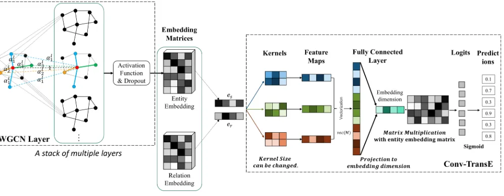
Figure 1: An illustration of our end-to-end Structure-Aware Convolutional Networks model. For encoder, a stack of multiple WGCN layers builds an entity/node embedding matrix. For decoder,esanderare fed intoConv-TransE. The output embeddings are vectorized and projected, and matched with all candidateeoembeddings via inner products. A logistic sigmoid function is used to get the scores.

18 billion edges (Ying et al. 2018). This success paves the way for a new generation of web-scale recommender sys-tems based on GCNs. Therefore we believe that our pro-posed model could take advantage of huge graph structures and high computational efficiency ofConv-TransE.

Method

In this section, we describe the proposed end-to-endSACN. The encoderWGCNis focused on representing entities by aggregating connected entities as specified by the relations in the KB. With node embeddings as the input, the decoder

Conv-TransEnetwork aims to represent the relations more accurately by recovering the original triplets in the KB. Both encoder and decoder are trained jointly by minimizing the discrepancy (cross-entropy) between the embeddingses+er andeoto preserve the translational propertyes+er ≈eo. We consider an undirected graph G = (V, E)throughout this section, whereV is a set of nodes with|V| =N, and E⊆V ×V is a set of edges with|E|=M.

Weighted Graph Convolutional Layer

The WGCN is an extension of classic GCN (Kipf and Welling 2016b) in the way that it weighs the different types of relations differently when aggregating and the weights are adaptively learned during the training of the network. By this adaptation, theWGCNcan control the amount of informa-tion from neighboring nodes used in aggregainforma-tion. Roughly speaking, theWGCNtreats a multi-relational KB graph as multiple single-relational subgraphs where each subgraph entails a specific type of relations. TheWGCNdetermines how much weights to give to each subgraph when combin-ing the GCN embeddcombin-ings for a node.

Thel-thWGCNlayer takes the output vector of lengthFl for each node from the previous layer as inputs and

gener-ates a new representation comprisingFl+1elements. Lethl_i represent the input (row) vector of the node vi in the l-th layer, and thus Hl _∈

RN×F

l

be the input matrix for this layer. The initial embedding H1 _{is randomly drawn from} Gaussian. If there are a total ofLlayers in theWGCN, the outputHL+1 _{of the}_L_{-th layer is the final embedding. Let} the total number of edge types beT in a multi-relational KB graph withE edges. The interaction strength between two adjacent nodes is determined by their relation type and this strength is specified by a parameter{αt,1 ≤ t ≤ T} for each edge type, which is automatically learned in the neural network.

Figure 1 illustrates the entire process ofSACN. In this ex-ample, theWGCN layers of the network compute the em-beddings for the red node in the middle graph. These lay-ers aggregate the embeddings of neighboring entity nodes as specified in the KB relations. Three colors (blue, yellow and green) of the edges indicate three different relation types in the graph. The corresponding three entity nodes are summed up with different weights according toαtin this layer to ob-tain the embedding of the red node. The edges with the same color (same relation type) use the sameαt. Each layer has its own set of relation weightsαtl. Hence, the output of the l-th layer for the nodevican be written as follows:

hl_i+1=σ



 X

j∈Ni

αltg(hli, hlj)



, (1)

wherehl j ∈ RF

l

(4)

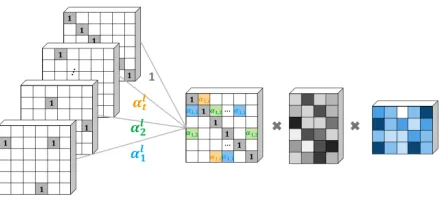
frame-Figure 2: A weighted graph convolutional network (WGCN) for entity embedding.

work, we implement the followinggfunction:

g(hl_i, hl_j) =hl_jWl, (2)

whereWl_∈

RF

l_×Fl+1

is the connection coefficient matrix and used to linearly transformhl

itoh l+1 i ∈R

Fl+1 .

In Eq. (1), the input vectors of all neighboring nodes are summed up but not the nodevi itself, hence self-loops are enforced in the network. For nodevi, the propagation pro-cess is defined as:

hl_i+1=σ(X

j∈Ni

αl_thl_jWl+hl_iWl). (3)

The output of the layerl is a node feature matrix:Hl+1 _∈

RN×F

l+1

, andhl_i+1 is the i-th row ofHl+1_{, which} repre-sents features of the nodeviin the(l+ 1)-th layer.

The above process can be organized as a matrix multi-plication as shown in Figure 2 to simultaneously compute embeddings for all nodes through an adjacency matrix. For each relation (edge) type, an adjacency matrixAtis a binary matrix whoseij-th entry is 1 if an edge connectingviandvj exists or 0 otherwise. The final adjacency matrix is written as follows:

Al=

T

X

t=1

(αl_tAt) +I, (4)

whereI is the identity matrix of size N ×N. Basically, the Al _{is the weighted sum of the adjacency matrices of} subgraphs plus self-connections. In our implementation, we consider all first-order neighbors in the linear transformation for each layer as shown in Figure 2:

Hl+1=σ(AlHlWl). (5)

Node Attributes. In a KB graph, nodes are of-ten associated with several attributes in the form of

(entity, relation, attribute). For example, (s=Tom,r=

people.person.gender,a =male) is an instance where gen-der is an attribute associated with a person. If a vector representation is used for node attributes, there would be two potential problems. First, the number of attributes for each node is usually small, and differs from one to another. Hence, the attribute vector would be very sparse. Second, the value of zero in the attribute vectors may have ambigu-ous meanings: the node does not have the specific attribute,

or the node misses the value for this attribute. These zeros would affect the accuracy of the embedding.

In this work, the entity attributes in the knowledge graph are represented by another set of nodes in the network called attribute nodes. Attribute nodes act as the “bridges” to link the related entities. The entity embeddings can be trans-ported over these “bridges” to incorporate the entity’s at-tribute into its embedding. Because these atat-tributes exhibit in triplets, we represent the attributes similarly to the repre-sentation of the entityoin relation triplets. Note that each type of attribute corresponds to a node. For instance, in our example, gender is represented by a single node rather than two nodes for “male” and “female”. In this way, theWGCN

not only utilizes the graph connectivity structure (relations and relation types), but also leverages the node attributes (a kind of graph structure) effectively. That is why we name ourWGCNas a structure-aware convolution network.

Conv-TransE

We develop the Conv-TransE model as a decoder that is based on ConvE but with the translational property of

TransE:es+er ≈eo. The key difference of our approach fromConvEis that there is no reshaping after stackingesand er. Filters (or kernels) of size2×k,k ∈ {1,2,3, ...}, are used in the convolution. The example in Figure 1 uses2×3

kernels to compute 2D convolutions. We experimented with several of such settings in our empirical study.

Note that in the encoder of SACN, the dimension of the relation embedding is commonly chosen to be the same as the dimension of the entity embedding, so in other words, is equal to FL. Hence, the two embeddings can be stacked. For the decoder, the inputs are two embedding matrices: oneRN×F

L

fromWGCNfor all entity nodes, and the other

RM×F

L

for relation embedding matrix which is trained as well. Because we use a mini-batch stochastic training algo-rithm, the first step of the decoder performs a look-up oper-ation upon the embedding matrices to retrieve the inputes anderfor the triplets in the mini-batch.

More precisely, givenCdifferent kernels where thec-th kernel is parameterized byωc, the convolution in the decoder is computed as follows:

mc(es, er, n) = K−1

X

τ=0

ωc(τ,0)ˆes(n+τ)

+ωc(τ,1)ˆer(n+τ),

(6)

(5)

Table 1: Scoring functionψ(es, eo). Heree¯sande¯rdenote a 2D reshaping ofesander.

Model Scoring Functionψ(es, eo) TransE ||es+er−eo||p DistMult < es, er, eo> ComplEx < es, er, eo>

ConvE f(vec(f(concat( ¯es,e¯r)∗ω))W)eo

ConvKB concat(g([es, er, eo]∗ω))β SACN f(vec(M(es, er))W)eo

[mc(es, er,0), ..., mc(es, er, FL−1)]. Aligning the output vectors from the convolution with all kernels yield a matrix

M(es, er)∈RC×F

L .

Finally, the scoring function for theConv-TransEmethod after the nonlinear convolution is defined as below:

ψ(es, eo) =f(vec(M(es, er))W)eo, (7)

whereW ∈RCF

L_×FL

is a matrix for the linear transforma-tion, andf denotes a non-linear function. The feature map matrix is reshaped into a vectorvec(M)∈ _RCFL _and pro-jected into aFLdimensional space usingWfor linear trans-formation. Then the calculated embedding is matched toeo by an appropriate distance metric. During the training in our experiments, we apply the logistic sigmoid function to the scoring:

p(es, er, eo) =σ(ψ(es, eo)). (8) In Table 1, we summarize the scoring functions used by several state of the art models. The vectoresandeoare the subject and object embedding respectively,eris the relation embedding, “concat” means concatenates the inputs, and “*” denotes the convolution operator.

In summary, the proposedSACNmodel takes advantage of knowledge graph node connectivity, node attributes and relation types. The learnable weights inWGCNhelp to col-lect adaptive amount of information from neighboring graph nodes. The entity attributes are added as additional nodes in the network and are easily integrated into theWGCN. Conv-TransEkeeps the translational property between entities and relations to learn node embeddings for the link prediction. We also emphasize that ourSACNhas significant improve-ments overConvEwith or without the use of node attributes.

Experiments

Benchmark Datasets

Three benchmark datasets (FB15k-237, WN18RR and FB15k-237-Attr) are utilized in this study to evaluate the performance of link prediction.

FB15k-237. The FB15k-237 (Toutanova and Chen 2015) dataset contains knowledge base relation triples and textual mentions of Freebase entity pairs, as used in the work published in (Toutanova and Chen 2015). The knowledge base triples are a subset of the FB15K (Bordes et al. 2013), originally derived from Freebase. The inverse relations are

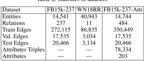
Table 2: Statistics of datasets.

Dataset FB15k-237 WN18RR FB15k-237-Attr

Entities 14,541 40,943 14,744

Relations 237 11 484

Train Edges 272,115 86,835 350,449

Val. Edges 17,535 3,034 17,535

Test Edges 20,466 3,134 20,466

Attributes Triples — — 78,334

Attributes — — 203

removed in FB15k-237.

WN18RR.WN18RR (Dettmers et al. 2017) is created from WN18 (Bordes et al. 2013), which is a subset of WordNet. WN18 consists of 18 relations and 40,943 entities. However, many text triples obtained by inverting triples from the training set. Thus WN18RR dataset (Dettmers et al. 2017) is created to ensure that the evaluation dataset does not have inverse relation test leakage. In summary, WN18RR dataset contains 93,003 triples with 40,943 entities and 11 relation types.

Data Construction

Most of the previous methods only model the entities and relations, and ignore the abundant entity attributes. Our method can easily model a large number of entity attribute triples. In order to prove the efficiency, we extract the attribute triples from the FB24k (Lin, Liu, and Sun 2016) dataset to build the evaluation dataset called FB15k-237-Attr.

FB24k. FB24k (Lin, Liu, and Sun 2016) is built based on Freebase dataset. FB24k only selects the entities and relations which constitute at least 30 triples. The number of entities is 23,634, and the number of relations is 673. In addition, the reversed relations are removed from the original dataset. In the FB24k datasets, the attribute triples are provided. FB24k contains 207,151 attribute triples and 314 attributes.

FB15k-237-Attr.We extract the attribute triples of entities in FB15k-237 from FB24k. During the mapping, there are 7,589 nodes from the original 14,541 entities which have the node attributes. Finally, we extract 78,334 attribute triples from FB24k. These triples include 203 attributes and 247 relations. Based on these triples, we create the “FB15k-237-Attr” dataset, which includes 14,541 entity nodes, 203 attribute nodes, 484 relation types. All the 78,334 attribute triples are combined with the training set of FB15k-237.

Experimental Setup

The hyperparameters in our Conv-TransE and SACN

(6)

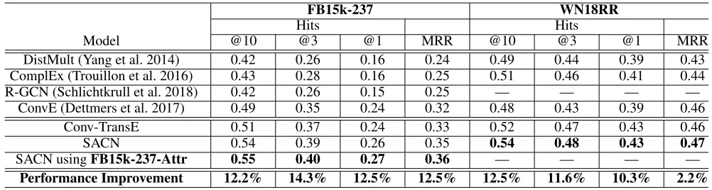
Table 3: Link prediction for FB15k-237, WN18RR and FB15k-237-Attr datasets.

FB15k-237 WN18RR

Hits Hits

Model @10 @3 @1 MRR @10 @3 @1 MRR

DistMult (Yang et al. 2014) 0.42 0.26 0.16 0.24 0.49 0.44 0.39 0.43

ComplEx (Trouillon et al. 2016) 0.43 0.28 0.16 0.25 0.51 0.46 0.41 0.44

R-GCN (Schlichtkrull et al. 2018) 0.42 0.26 0.15 0.25 — — — —

ConvE (Dettmers et al. 2017) 0.49 0.35 0.24 0.32 0.48 0.43 0.39 0.46

Conv-TransE 0.51 0.37 0.24 0.33 0.52 0.47 0.43 0.46

SACN 0.54 0.39 0.26 0.35 0.54 0.48 0.43 0.47

SACN usingFB15k-237-Attr 0.55 0.40 0.27 0.36 — — — —

Performance Improvement 12.2% 14.3% 12.5% 12.5% 12.5% 11.6% 10.3% 2.2%

{100,200,300}, number of kernels {50,100,200,300}, and kernel size{2×1,2×3,2×5}.

Here all the models use theWGCNwith two layers. For different datasets, we have found that the following settings work well: for FB15k-237, set the dropout to 0.2, number of kernels to 100, learning rate to 0.003 and embedding size to 200 forSACN; for WN18RR dataset, set dropout to 0.2, number of kernels to 300, learning rate to 0.003, and embed-ding size to 200 forSACN. When using theConv-TransE -alone model, these settings still work well.

Each dataset is split into three sets for: training, valida-tion and testing, which is same with the setting of the origi-nalConvE. We use the adaptive moment (Adam) algorithm (Kingma and Ba 2014) for training the model. Our models are implemented by PyTorch and run on NVIDIA Tesla P40 Graphics Processing Units. For the FB15k-237 dataset, the computation time ofSACNfor each epoch is about 1 minute. For the WN18RR, the computation time ofSACNfor one epoch is about 1.5 minutes.

Results

Evaluation Protocol Our experiments use the the propor-tion of correct entities ranked in top 1,3 and 10 (Hits@1, Hits@3, Hits@10) and the mean reciprocal rank (MRR) as the metrics. In addition, since some corrupted triples exist in the knowledge graphs, we use the filtered setting (Bordes et al. 2013), i.e. we filter out all valid triples before ranking.

Link Prediction Our results on the standard FB15k-237, WN18RR and FB15k-237-Attr are shown in Table 3. Ta-ble 3 reports Hits@10, Hits@3, Hits@1 and MRR results of four different baseline models and two our models on three knowledge graphs datasets. The FB15k-237-Attr dataset is used to prove the efficiency of node attributes. So we run our SACN in FB15k-237-Attr to do the comparison with SACN using FB15k-237.

We first compare ourConv-TransE model with the four baseline models.ConvEhas the best performance compar-ing all baselines. In FB15k-237 dataset, our Conv-TransE

model improves upon ConvE’s Hits@10 by a margin of 4.1% , and upon ConvE’s Hits@3 by a margin of 5.7% for the test. In WN18RR dataset,Conv-TransEimproves upon ConvE’s Hits@10 by a margin of 8.3% , and upon ConvE’s

Hits@3 by a margin of 9.3% for the test. For these results, we conclude thatConv-TransEusing neural network keeps the translational characteristic between entities and relations and achieve better performance.

Second, the structure information is added into ourSACN

model. In Table 3,SACNalso get the best performances in the test dataset comparing all baseline methods. In FB15k-237, comparingConvE, ourSACNmodel improves Hits@10 value by a margin of 10.2%, Hits@3 value by a margin of 11.4%, Hits@1 value by a margin of 8.3% and MRR value by a margin of 9.4% for the test. In WN18RR dataset, com-paringConvE, ourSACNmodel improves Hits@10 value by a margin of 12.5%, Hits@3 value by a margin of 11.6%, Hits@1 value by a margin of 10.3% and MRR value by a margin of 2.2% for the test. So our method has significant improvements overConvEwithout attributes.

Third, we add node attributes into ourSACNmodel, i.e. we use the FB15k-237-Attr to trainSACN. Note thatSACN

has significant improvements over ConvE without attributes. Adding attributes improves performance again. Our model using attributes improves upon ConvE’s Hits@10 by a mar-gin of 12.2% , Hits@3 by a marmar-gin of 14.3%, Hits@1 by a margin of 12.5% and MRR by a margin of 12.5%. In ad-dition, our SACNusing attributes improved Hits@10 by a margin of 1.9% , Hits@3 by a margin of 2.6%, Hits@1 by a margin of 3.8% and MRR by a margin of 2.9% comparing withSACNwithout attributes.

In order to better compare with ConvE, we also use the attributes intoConvE. Here the attributes will be treated as the entity triplets. Following the official ConvE code with default setting, the test result in FB15k-237-Attr was: 0.46 (Hits@10), 0.33 (Hits@3), 0.22 (Hits@1) and 0.30 (MRR). Comparing to the performance without the attributes, adding the attributes into theConvEdidn’t improve performance.

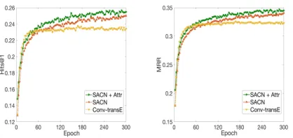
Convergence Analysis Figure 3 shows the convergence of the three models. We can see that theSACN(the red line) is always better thanConv-TransE(the yellow line) after sev-eral epochs. And the performance of SACNkeeps increas-ing after around 120 epochs. However, the Conv-TransE

(7)

Figure 3: The convergence study of SACN, Conv-TransE

models in FB15k-237 andSACNin FB15k-237-Attr (SACN + Attr) using the validation set. Due to the page limitation, only the results of Hits@1 and MRR are reported here.

Table 4: Kernel size analysis for 237 and FB15k-237-Attr datasets. “SACN+Attr” means the SACN using FB15k-237-Attr dataset.

FB15k-237

Hits

Model Kernel Size @10 @3 @1 MRR

Conv-TransE 2×1 0.504 0.357 0.234 0.324 Conv-TransE 2×3 0.513 0.365 0.240 0.331 Conv-TransE 2×5 0.512 0.361 0.239 0.329

SACN 2×1 0.527 0.379 0.255 0.345

SACN 2×3 0.536 0.384 0.260 0.351

SACN 2×5 0.536 0.385 0.261 0.352

SACN+Attr 2×1 0.535 0.384 0.260 0.351

SACN+Attr 2×3 0.543 0.394 0.268 0.360

SACN+Attr 2×5 0.547 0.396 0.268 0.360

dataset, the performance of “SACN + Attr” is better than “SACN” model.

Kernel Size Analysis In Table 4, different kernel sizes are examined in our models. The kernel of “2×1” means the knowledge or information translating between one at-tribute of entity vector and the corresponding atat-tribute of re-lation vector. If we increase the kernel size to “2×k” where k = {3,5}, the information is translated between a com-bination ofs attributes in entity vector and a combination ofkattributes in relation vector. The larger view to collect attribute information can help to increase the performance as shown in Table 4. All the values of Hits@1, Hits@3, Hits@10 and MRR can be improved by increasing the kernel size in the FB15k-237 and FB15k-237-Attr datasets. How-ever, the optimal kernel size may be task dependent.

Node Indegree Analysis The indegree of the node in knowledge graph is the number of edges connected to the node. The node with larger degree means it have more neigh-boring nodes, and this kind of nodes can receive more in-formation from neighboring nodes than other nodes with smaller degree. As shown in Table 5, we present the results for different sets of nodes with different indegree scopes. The average Hits@10 and Hits@3 scores are calculated.

Table 5: Node indegree study using FB15k-237 dataset.

Conv-TransE SACN

Average Hits Average Hits

Indegree Scope @10 @3 @10 @3

[0,100] 0.192 0.125 0.195 0.134

[100,200] 0.441 0.245 0.441 0.253

[200,300] 0.696 0.446 0.705 0.429

[300,400] 0.829 0.558 0.806 0.577

[400,500] 0.894 0.661 0.868 0.663

[500,1000] 0.918 0.767 0.891 0.695

[1000, maximum] 0.992 0.941 0.981 0.922

Along the increasing of indegree scope, the average value of Hits@10 and Hits@3 will be increased. First for a node with small indegree, it benefits from aggregation of neighbor information from the WGCN layers ofSACN. Its embedding can be estimated robustly. Second for a node with high in-degree, it means that a lot more information is aggregated through GCN, and the estimation of its embedding is sub-stantially smoothed among neighbors. Thus the embedding learned from SACN is worse than that fromConv-TransE. One solution to this problem would be neighbor selection as in (Ying et al. 2018).

Conclusion and Future Work

We have introduced an end-to-end structure-aware convolu-tional network (SACN). The encoding network is a weighted graph convolutional network, utilizing knowledge graph connectivity structure, node attributes and relation types.

WGCN with learnable weights has the benefit of collect-ing adaptive amount of information from neighborcollect-ing graph nodes. In addition, the entity attributes are added as the nodes in the network so that attributes are transformed into knowledge structure information, which is easily integrated into the node embedding. The scoring network ofSACNis a convolutional neural model, calledConv-TransE. It uses a convolutional network to model the relationship as the trans-lation operation and capture the transtrans-lational characteristic between entities and relations. We also prove that Conv-TransEalone has already achieved the state of the art per-formance. The performance ofSACNachieves overall about 10% improvement than the state of the art such asConvE.

In the future, we would like to incorporate the neighbor selection idea into our training framework, such as, impor-tance pooling in (Ying et al. 2018) which takes into account the importance of neighbors when aggregating the vector representations of neighbors. We would also like to extend our model to be scalable with larger knowledge graphs en-couraged by the results in (Ying et al. 2018).

Acknowledgements

(8)

References

Auer, S.; Bizer, C.; Kobilarov, G.; Lehmann, J.; Cyganiak, R.; and Ives, Z. 2007. Dbpedia: A nucleus for a web of open data. InThe semantic web. Springer. 722–735.

Bollacker, K.; Evans, C.; Paritosh, P.; Sturge, T.; and Taylor, J. 2008. Freebase: a collaboratively created graph database for structuring human knowledge. In Proceedings of the 2008 ACM SIGMOD international conference on Manage-ment of data, 1247–1250. AcM.

Bordes, A.; Usunier, N.; Garcia-Duran, A.; Weston, J.; and Yakhnenko, O. 2013. Translating embeddings for model-ing multi-relational data. InAdvances in neural information processing systems, 2787–2795.

Bruna, J.; Zaremba, W.; Szlam, A.; and LeCun, Y. 2013. Spectral networks and locally connected networks on graphs.arXiv preprint arXiv:1312.6203.

Carlson, A.; Betteridge, J.; Kisiel, B.; Settles, B.; Hr-uschka Jr, E. R.; and Mitchell, T. M. 2010. Toward an architecture for never-ending language learning. In AAAI, volume 5, 3. Atlanta.

Defferrard, M.; Bresson, X.; and Vandergheynst, P. 2016. Convolutional neural networks on graphs with fast localized spectral filtering. InAdvances in Neural Information Pro-cessing Systems, 3844–3852.

Dettmers, T.; Minervini, P.; Stenetorp, P.; and Riedel, S. 2017. Convolutional 2d knowledge graph embeddings.

arXiv preprint arXiv:1707.01476.

Hamilton, W.; Ying, Z.; and Leskovec, J. 2017a. Induc-tive representation learning on large graphs. InAdvances in Neural Information Processing Systems, 1025–1035. Hamilton, W. L.; Ying, R.; and Leskovec, J. 2017b. Rep-resentation learning on graphs: Methods and applications.

Henaff, M.; Bruna, J.; and LeCun, Y. 2015. Deep convo-lutional networks on graph-structured data. arXiv preprint arXiv:1506.05163.

Ji, G.; He, S.; Xu, L.; Liu, K.; and Zhao, J. 2015. Knowledge graph embedding via dynamic mapping matrix. In Proceed-ings of the 53rd Annual Meeting of the Association for Com-putational Linguistics and the 7th International Joint Con-ference on Natural Language Processing (Volume 1: Long Papers), volume 1, 687–696.

Kingma, D. P., and Ba, J. 2014. Adam: A method for stochastic optimization.arXiv preprint arXiv:1412.6980. Kipf, T. N., and Welling, M. 2016a. Variational graph auto-encoders. InAdvances in neural information processing sys-tems,Bayesian Deep Learning Workshop.

Kipf, T. N., and Welling, M. 2016b. Semi-supervised clas-sification with graph convolutional networks.arXiv preprint arXiv:1609.02907.

Lin, Y.; Liu, Z.; Sun, M.; Liu, Y.; and Zhu, X. 2015. Learn-ing entity and relation embeddLearn-ings for knowledge graph completion. InAAAI, volume 15, 2181–2187.

Lin, Y.; Liu, Z.; and Sun, M. 2016. Knowledge

representa-tion learning with entities, attributes and relarepresenta-tions. ethnicity

1:41–52.

Mahdisoltani, F.; Biega, J.; and Suchanek, F. M. 2013. Yago3: A knowledge base from multilingual wikipedias. In

CIDR.

Nguyen, D. Q.; Sirts, K.; Qu, L.; and Johnson, M. 2016. Stranse: a novel embedding model of entities and relation-ships in knowledge bases.arXiv preprint arXiv:1606.08140. Nguyen, D. Q.; Nguyen, T. D.; Nguyen, D. Q.; and Phung, D. 2017. A novel embedding model for knowledge base completion based on convolutional neural network. arXiv preprint arXiv:1712.02121.

Nguyen, D. Q. 2017. An overview of embedding models of entities and relationships for knowledge base completion.

Pham, T.; Tran, T.; Phung, D.; and Venkatesh, S. 2017. Col-umn networks for collective classification.

Schlichtkrull, M.; Kipf, T. N.; Bloem, P.; van den Berg, R.; Titov, I.; and Welling, M. 2018. Modeling relational data with graph convolutional networks. InEuropean Semantic Web Conference, 593–607. Springer.

Shang, C.; Liu, Q.; Chen, K.-S.; Sun, J.; Lu, J.; Yi, J.; and Bi, J. 2018. Edge attention-based multi-relational graph convolutional networks. arXiv preprint arXiv:1802.04944. Sharma, A.; Talukdar, P.; et al. 2018. Towards understanding the geometry of knowledge graph embeddings. In Proceed-ings of the 56th Annual Meeting of the Association for Com-putational Linguistics (Volume 1: Long Papers), volume 1, 122–131.

Toutanova, K., and Chen, D. 2015. Observed versus latent features for knowledge base and text inference. In Proceed-ings of the 3rd Workshop on Continuous Vector Space Mod-els and their Compositionality, 57–66.

Trouillon, T.; Welbl, J.; Riedel, S.; Gaussier, ´E.; and Bouchard, G. 2016. Complex embeddings for simple link prediction. InInternational Conference on Machine Learn-ing, 2071–2080.

Wang, Z.; Zhang, J.; Feng, J.; and Chen, Z. 2014. Knowl-edge graph embedding by translating on hyperplanes. In

AAAI, volume 14, 1112–1119.

Wang, Q.; Mao, Z.; Wang, B.; and Guo, L. 2017. Knowl-edge graph embedding: A survey of approaches and appli-cations. IEEE Transactions on Knowledge and Data Engi-neering29(12):2724–2743.