A Powerful Global Test Statistic for Functional Statistical Inference

(1)

The Thirty-Third AAAI Conference on Artificial Intelligence (AAAI-19)

A Powerful Global Test Statistic for Functional Statistical Inference

Jingwen Zhang,

1

_{Joseph Ibrahim,}

1

_{Tengfei Li,}

2

_{Hongtu Zhu}

1 1_{Department of Biostatistics, UNC Gillings School of Global Public Health}

2_{Biomedical Research Imaging Center, UNC School of Medicine}

University of North Carolina at Chapel Hill [email protected], [email protected] [email protected], [email protected]

Abstract

We consider the problem of performing an association test between functional data and scalar variables in a varying co-efficient model setting. We propose a functional projection regression model and an associated global test statistic to ag-gregate relatively weak signals across the domain of functional data, while reducing the dimension. An optimal functional pro-jection direction is selected to maximize signal-to-noise ratio with ridge penalty. Theoretically, we systematically study the asymptotic distribution of the global test statistic and provide a strategy to adaptively select the optimal tuning parameter. We use simulations to show that the proposed test outperforms all existing state-of-the-art methods in functional statistical inference. Finally, we apply the proposed testing method to the genome-wide association analysis of imaging genetic data in UK Biobank dataset.

Introduction

Functional regression modeling with a functional response

y(s), s ∈ S and multivariate covariates x ∈ _Rp _{is a} powerful statistical tool in modern high-dimensional infer-ence, with wide applications in various biomedical stud-ies. Specifically, functional responses frequently arise in medical imaging, computational biology and computer vi-sion, and have been widely used to characterize brain structure and function, such as cortical complexity and white matter microstructure (Grenander and Miller 2007; Miller and Qiu 2009; Kendall et al. 2009; Srivastava and Klassen 2016; Smith et al. 2006; Smith and Nichols 2009; Huang et al. 2017). In imaging genetic studies, our primary problem of interest is to identify genetic variants (x) associ-ated with functional phenotypic variation (y(s)), which may ultimately lead to discoveries of risk genes contributing to neuropsychiatric and neurological disorders.

Suppose that we observe a functional responseyi(s)and a set of clinical variables (e.g., age, genetic markers, and gender)xi ∈ Rpfornunrelated subjects. Without loss of generality, we assume S = [0, S] for a positive scalar S. Throughout this paper, we considernindependent observa-tions(yi(s),xi)and a varying coefficient model given by

yi(s) =xTiβ(s) +ηi(s) +ei(s), (1)

whereβ(s)is ap×1vector of functional coefficients,ηi(s) is a function of random effect that characterizes subject-specific spatial variation, and ei(s) represents measure-ment error. It is assumed thatηi(s)andei(s)are mutually independent and identical copies of SP{0,Ση(s, s0)} and SP{0, σ2

e(s)I(s = s0)}, respectively, where SP(µ,Σ) de-notes a stochastic process with mean functionµ(s)and co-variance functionΣ(s, s0), andI(·)is the indicator function of an event. Many hypothesis testing problems of interest, such as comparison across groups, can often be formulated as a global testing problem acrossS, which is given by,

H0: Cβ(s) =b0(s) ∀s∈ S,

H1: Cβ(s)=6 b0(s) ∃s∈ S, (2)

in whichCis anr×pmatrix andb0(s)is anr×1matrix. Without loss of generality, we center the covariates, stan-dardize the responses, and assume rank(C) = r = 1and

b0(s) =0.

The key problem is how to design a powerful global test statistic that can efficiently aggregate weak signals across

S, while achieving high statistical power for testing prob-lem (2). To the best of our knowledge, such probprob-lem has not been fully solved yet. We focus on a specific setting that all components inβ(s)lie in an infinite-dimensional functional space, butpis relatively small. Existing testing methods are not powerful enough to detect moderate or weak signals due to two major challenges, (i) infinite-dimensional functional parameters and (ii) complicated covariance struc-ture Ση(s, s0). Popular pooled global test statistics are to conduct univariate analysis at each sample grid point ofS

(2)

prob-lem. Finally, some recent developments in regularization methods, such as multiple task learning, do not provide a post-inference tool, e.g.,p-values, (Sun, Ji, and Ye 2016; Trevor, Tibshirani, and Friedman 2009).

The proposed method has three major contributions given as follows:

• A novel functional projection regression model and its associated global test statistic are introduced to aggregate relatively weak signals acrossS, while reducing the dimen-sion of functional data. An optimal functional projection direction is calculated by maximizing statistical power with ridge penalty.

• The asymptotic distribution of the global test statistic is studied systematically under both null and alternative hy-potheses and a data-driven strategy is provided to adap-tively select the optimal tuning parameter.

• Numerical simulations show that the proposed test outper-forms all existing state-of-the-art methods in functional statistical inference.

The rest of the paper is organized as follows. We first introduce a functional projection model and the associated global test statistic for testing problem (2). Next, we derive the asymptotic distribution of the test statistic under both null and alternative hypotheses. Finally we use numerical simulations and a real data example to examine the finite sample performance of the global test statistic and conclude with some remarks.

Method

Functional Projection Regression Model

We propose a functional projection regression model as fol-lows. Specifically, letω(s)be a weight function inL2(S), we define the following pseudo responseyw,i, which is a projected variable onto the functional directionω(s)given as

yw,i

∆

=xT_iβ_w+ηw,i(s), (3)

where β_w =

Z

S

β(s)ω(s)ds, andηw,i = Z

S

ηi(s)ω(s)ds.

The term associated withei(s)in (3) would converges to 0 in probability through local kernel smoothing and therefore is asymptotically ignorable. The projected model (3) transforms the functional data into a univariate variableyw,i. Letβb_wand

b

Ση(s, s0)be the estimates ofβwandΣη(s, s0)respectively, then a standard Wald-type statistic for testing problem (2) can be given by

Tn(ω) = b

βT_wCT_[_C₍_XT_X₎−1_CT_]−1_C

b

β_w

Z Z

b

Ση(s, s0)ω(s)ω(s0)dsds0

. (4)

For a given projection direction ofω(s), we need to esti-mateβb(s)andΣbη(s, s0)in order to calculateTn(ω). In real data, functional responses{yi(s)}ni=1are usually observed

on a set ofM discrete sample points onS, which is denoted asSb={s1,· · · , sm,· · · , sM}. To estimateβ(s), we use a weighted least square (WLS) method based on the local poly-nomial kernel (LPK) smoothing technique (Fan and Gijbels

2018; Zhu, Li, and Kong 2012). LetK(s)be a predetermined smoothing kernel on[−1,1]and letKh(s) = h−1K(s/h) for bandwidthh. A smooth estimate ofβ(s)can be given as the minimizers of the following weighted least square function given by

b

β_h

1(s) = argmin β(s)

n X

i=1

Kh1[yi(s),x

T

iβ(s)|Sb], (5)

whereKh1[yi(s),x

T

iβ(s)|Sb]is defined as M

X

m=1

[yi(sm)−xTiβ(s)]

2_K

h1(sm−s). (6)

Similarly, each random functionηi(s)can also be estimated by

b

ηi,h2(s) = argmin

ηi(s)

Kh2[yi(s)−x

T

iβb_h₁(s), ηi(s)|Sb], (7)

whereKh2[yi(s)−x

T

i βb_h₁(s), ηi(s)|Sb]is defined as

M X

m=1

[yi(sm)−xTiβb_h

1(sm)−ηi(s)] 2_K

h2(sm−s). (8)

With{η_bi,h2(s)}

n

i=1, we can obtain a consistent estimate of

Ση(s, s0)as

b

Ση(s, s0) =

1 n n X i=1 b

ηi,h2(s)bηi,h2(s

0₎_. ₍₉₎

Finally, we address the problem of determiningω(s)in order to achieve optimal power. Specifically, we consider the signal-to-noise ratio of test statisticsTn(ω), which dominates the asymptotic power, as follows:

L1(ω) =

βT_wCT_[_C₍_XT_X₎−1_CT_]−1_C_β

w Z Z

Ση(s, s0)ω(s)ω(s0)dsds0

. (10)

An optimal projection direction would be the maximizer of

L1(ω). However, when plugging in the estimates ofβ(s)

and Ση(s, s0), directly maximizing L1(ω) can be an

ill-conditioned problem. The eigenvalues ofΣbη(s, s0)usually decrease to zero very fast and the maximum value ofL1(w)

tend to be∞. To solve this issue, we add a ridge penalty term to the denominator in (10). Given a positive tuning parameter

λ, the optimal projection directionω_bλ(s)can be estimated as

argmax

ω(s)

b

βTw,h1C

T_[_C₍_XT_X₎−1_CT_]−1_C

b

βw,h1

Z Z

b

Ση(s, s0)ω(s)ω(s0)dsds0+λkω(s)k22

, (11)

wherekω(s)k2 2=

R

Sω

2₍_s₎_ds_{is the}_L 2-norm.

For a givenλ, we calculateω_bλ(·)as follows. Let{τbk}

+∞

k=1

be the eigenvalues of Σbη(s, s0)in a decreasing order and let {φbk(s)}+∞k=1 be the corresponding eigenfunctions. We

(3)

ω(s) =P+∞

k=1wkφk(s). In that case, we can seek solution

b

ωλ(s)in the space spanned by{φbk(s)}+∞k=1, which is given

by

b

wλ = (wb1,λ,· · ·,wbk,λ,· · ·)

= argmax

w1,···,wk,···

[P+∞

k=1dbk,h1wk] 2

P+∞ k=1w

2

k(bτk+λ)

, (12)

where

b

wk,λ = Z S

0 b

ωλ(s)φbk(s)ds and

b

dk,h1 =

Z S

0

Cβb_h₁(s)φbk(s)ds

are the projections of functional direction ω_bλ(s) and es-timated signal Cβb_h₁(s) on the estimated eigenfunctions

{φbk(s)}∞k=1 respectively. The solutions to (12) can be

ex-plicitly expressed as,

b

wk,λ =dbk,h1/(τbk+λ). (13)

Finally, we obtain a global test statistic based on the optimal projection directionω_bλ(s) =P+∞k=1wbk,λφbk(s)as follows:

Tn(ωbλ) =

(P+∞

k=1dbk,h1wbk,λ)

2

[C(XT_X₎−1_CT_]P+∞ k=1τbkwb

2

k,λ

. (14)

An unsolved question is how to choose the tuning parameter

λ, which will be answered in Section 3. To approximate the distribution ofTn(ω_bλ)underH0, we adopt a wild-boostrap

procedure described as follows.

Algorithm 1.

(a) Fit the varying coefficient model under the null hypothesis and get the estimate ofβb0(s)and{ηbi,0(s),bei,0(s)}

n i=1. (b) Forg = 1,· · ·, G, generate independent random num-bersν_i(g)andν_i(g)(sm)fromN(0,1), and the wild bootstrap sample on each grid point can be calculated as

b

y_i(g)(sm) =βb0(sm)Txi+ν

(g)

i ηbi,0(sm)+ν

(g)

i (sm)bei,0(sm). (c) Repeat the testing procedure and obtainGsamples of

Tn(bω

(g)

λ )under the null hypothesis. (d) Thep-value is approximated by

p=G−1

G X

g=1

I{Tn(w_bλ)≥Tn(ω_b

(g)

λ )}.

Approximation of the null distribution requires repeated calculation of the estimation-test procedure byGtimes, and

Gshould be large enough to guarantee accuracy.

Theoretical Result

In this section, we study the asymptotic distribution of the proposed test statisticTn(ω_bλ)for fixedλand consider the problem of determining the tuning parameterλfor optimally testing (2).

Assumptions

Throughout the paper, the following assumptions are used to facilitate the technical details. Some of the assumptions might be weakened but the current version simplifies the proof.

Assumption 1. Smoothing kernelK(u)is a symmetric posi-tive function with compact support[−1,1]and upper bound

c1. Moreover, K(u) has continuous first order derivative satisfyingsup_u|K˙(u)|< c2<+∞.

Assumption 2. Variable of interestxiare identically and in-dependently distributed variables with meanµxand positive definite covarianceΣx. Andkxik∞< c3<+∞.

Assumption 3. Sample grid point setSbis composed ofM equidistant points on[0, S].

Assumption 4. Fixed effectsβ(s)are continuous functions inC1_[0_{, S}_]_{with universally bounded first order derivatives,} i.e.,sup_skβ˙(s)k∞< c4<+∞.

Assumption 5. Random functions{ηi(s)}ni=1are identically and independently distributed copies from gaussian process and the sample path has continuous first-order derivative on

[0, S]. Additionally, it is assumed thatη˙i(s)is from gaussian process and its covariance function has continuous first-order derivatives, i.e.,Ση˙(s, t)∈C1[0, S]2.

Assumption 6. Error terms{ei(s)}ni=1are from a univer-sally upper bounded process, that is,sups|ei(s)| < c7 < +∞.

Assumption 7. Let Ση(s, s0) = P

+∞

k=1τkφk(s)φk(s0) be the spectral expansion of Ση(s, s0), in which τ1 > · · · >

τk > · · · ≥ 0 are eigenvalues in decreasing order. It is assumed that all eigenvalues have simple multiplicity that satisfy

min

k minj6=k|τj−τk|/τk > 0>0.

Let{λn}be a sequence of tuning parameters that satisfy

λn→0asn→+∞, we further assume that one of the two conditions holds,

(i) {τk}+∞k=1 follows polynomial decay rate, i.e.τk k−r

with r > 1, it is assumed that λ1−1r

n M h1 → +∞ and

λ3−

1

r

n min{h−2₁ , h−2₂ , M h2, n/logn} →+∞.

(ii){τk}+∞k=1follows exponential decay rate, i.e.τk α−k withα >1, it is assumed thatM h1λnlogλ−1n →+∞and

λ3

nlogλ−1n min{h

−2 1 , h

−2

2 , M h2, n/logn} →+∞.

Assumption 8(Local Alternative Hypothesis). A sequence of local alternative hypothesesH1n:Cβ(s) =n−1/2d0(s) is satisfied as n → +∞, where d0(s) ∈ C1[0, S] ∩ span{φk(s)}+∞k=1.

Assumptions 1-6 are standard conditions in functional data analysis (Zhu, Li, and Kong 2012; Hall, M¨uller, and Wang 2006; Li and Hsing 2010), which are required to guarantee that the estimates ofβ(s)andΣη(s, s0)are consistent. As-sumption 7 is required in order to specify the bound of tuning parameterλnfor two different decay rates of{τk}+∞k=1. These

(4)

Yuan and Cai 2010; Wang and Ruppert 2015). Here, we only consider distinct eigenvalues. And the distance between one eigenvalue and any other eigenvalues can not be too large compared to itself. Conclusions for multiplicity greater than one could be reached, yet is beyond the discussion of this paper. Assumption 8 specified a sequence of local alternative hypotheses from which we will derive the asymptotic power.

Main Theoretical Results

We present the key results below according to different de-cay rates of{τk}+∞k=1. The proof of the theorem is given in

https://app.box.com/v/aaai19PFGT.

Theorem 1. When Assumptions 1 - 6 and 7(i) (or 7(ii)) hold, asn, M → +∞,Tn(ω_bλn) has the following asymptotic

normal distribution under the null hypothesis,

Tn(ω_bλn) d

−→ N{µ0, σ20}, (15)

where−→d denotes convergence in distribution andµ0andσ20 are given by,

µ0=

a2 1

a2

and σ2₀=8a 2 1

a2 +2a

4 1a4

a4 2

−8a 3 1a3

a3 2

, (16)

in whicha1, a2, a3,anda4are defined as,

a1 = +∞

X

k=1

τk

τk+λn

, a2= +∞

X

k=1 ( τk

τk+λn

)2,

a3 = +∞

X

k=1 ( τk

τk+λn

)3, a4= +∞

X

k=1 ( τk

τk+λn

)4.

When Assumptions 1 - 6 and 7(i) (or 7(ii)) hold, and the local alternative hypothesis specified by Assumption 8 is satisfied,

Tn(bωλn)has the following asymptotic normal distribution

given by

Tn(ωbλn) d

−→ N{µ1, σ21}, (17)

whereµ1andσ21are defined as,

µ1 =

(a1+d1)2

a2+d2

,

σ₁2 = 8(a1+d1) 2₍_a

2+ 2d2) (a2+d2)2

+ 2(a1+d1) 4₍_a

4+ 2d4) (a2+d2)4

− 8(a1+d1) 3₍_a

3+ 2d3) (a2+d2)3

. (18)

In the above equation,d1, d2, d3,andd4are defined as

d1 = +∞ X k=1 δ2 k,0 σ2

c(τk+λn)

, d2= +∞

X

k=1

τkδk,20

σ2

c(τk+λn)2

,

d3 = +∞

X

k=1

τ2

kδ2k,0

σ2

c(τk+λn)3

, d4= +∞

X

k=1

τ3

kδk,20

σ2

c(τk+λn)4

,

whereδ0,k= Z S

0

d0(s)φk(s)dsandσc2=CΣ

−1

x CT.

Theorem 1 establishes the asymptotic distribution of the proposed test statistics for polynomial and exponential decay rates under both null and alternative hypotheses. It inspires a data-driven criterion to adaptively select tuning parameterλn in order to achieve optimal power. Specifically, we choose

b

λn = argmax[µ_b1/σ_b1−µ_b0/_bσ0], (19)

in which_bµ0,µb1,σb0,σb1are calculated by plugging in their corresponding estimates. Intuitively, (19) tends to maximize the asymptotic power ofTn(ωbλn)under alternative hypothe-sis.

Numerical Simulation

Setup

In this section, we use numerical simulations to evaluate the finite-sample performance of the proposed global test statistic. Data was generated from the following model

yi(s) =β0(s) +xi,1β1(s) +ηi(s) +ei(s), i= 1,· · ·n,

wherexi,1 ∼N(0,1). We setn= 200andS = 1and put

the number of grid pointsM = 100evenly in[0,1]. Our hypothesis of interest is to test the following problem:

H0:β1(s) = 0,∀s∈[0,1],

H1:β1(s)= 06 ,∃s∈[0,1].

In this experiment, we simulated β1(s)as a spatially

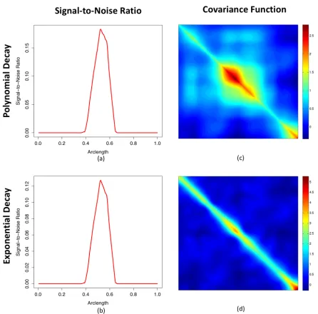
het-erogenous function under the alternative hypothesis. Other model parameters were estimated from the UK Biobank dataset introduced in Application Section. We considered two decay rates of{τk}+∞_k₌₁ including a polynomial decay rate withτk =k−3/2 and an exponential decay rate given byτk = 0.75k. The signal-to-noise ratios under alternative hypothesis are shown in Figure 1 (a)-(b) and the structure of the covariance functions are presented in Fig 1 (c)-(d). As can be seen, responses in the polynomial decay case have stronger spatial correlation than those in the exponential de-cay case. For the choice of the tuning parameter, we consid-ered both fixed quantities wherelogλn takes values from

[−2,0]with an equal increment of0.1 (PFGT-λn) and an optimalλbnselected by (19) in each run (PFGT-optimal). As a comparison, we considered two state-of-the-art methods in functional statistical inference, including FADTTS (Zhu, Li, and Kong 2012) and FLMtest (Zhang 2011). In each scenario, 1,000 simulation replicates were generated to evaluate type I and type II error rates respectively. To calculatep-values,

G= 1,000wild-bootstrap samples were generated in each run.

Results

(5)

Figure 1: Simulation settings: Panels (a)-(b) demonstrate the signal-to-noise ratios under alternative hypothesis. Panels (c)-(d) visualize the covariance function of simulated responses along the curve.

decay rate and the exponential decay rate. In addition, the proposed test using adaptive tuning parameterbλnachieves almost the best performance given by PFGT using fixedλn, which indicates the effectiveness of the data-driven strategy to chooseλn. Moreover, PFGT shows larger improvement in the polynomial decay case than in the exponential decay case compared with FADTTS and FLMtest. It is suggested that the proposed method has better performance in the presence of stronger spatial correlation.

Application: UK Biobank Data Analysis

UK Biobank Study

UK Biobank is a large-scale cohort in the United Kingdom designed to investigate the influences of genetic susceptibility, environmental exposures and lifestyle factors to a wide range of health-related outcomes and disorders in middle aged and elderly population. In this section, we perform a genome-wide association analysis on the functional neuroimaging phenotypes from this study.

Diffusion weighted images (DWI) were acquired for 8751 subjects in total. We ran the TBSS-ENIGMA pipeline (McMahon and Thompson 2017) on DWIs with the FSL tool set (Jenkinson et al. 2012) to perform quality control and registration. The ENIGMA skeleton was then projected onto the registered FA images and FA statistics on 26,334 vox-els from 21 regions of interest (ROIs) were obtained. The primary phenotype of interest is the distributional density of voxel-wise FA statistics of the whole brain. As the den-sity function is constrained by the normalization condition, we applied a log quantile density transformation introduced in (Petersen and M¨uller 2016) and took the output as the functional phenotypes for further analysis.

Figure 2: Simulation results: Panels (a)-(b) present the type I error for PFGT-λn, PFGT-optimal, FADTTS and FLMTest. Panels (c)-(d) present the power under alternative hypothesis.

The Affymetrix Axiom platform was used to genotype 8057 subjects from the full population with imaging data, which resulted in a set of 784,256 single-nucleotide poly-morphism (SNPs). The genotype data were preprocessed by standard quality control steps and SNPs with minor allele frequency (MAF) less than1%were removed. Eventually, 459,588 SNPs were remained in the dataset for further analy-sis.

Statistical Analysis and Results

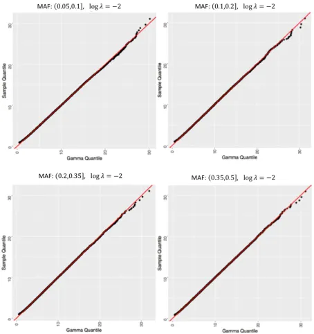
Our problem of interest is to perform a genome-wide asso-ciation analysis on the log quantile curve of the whole brain FA measure. We fitted model (1) with covariates including an intercept term, a specific SNP, age, gender, and the top 5 genetic principal components. We developed a computation-ally efficient strategy to approximate the p-values of SNPs with different MAFs. For each MAF category, we generated 10,000 bootstrap samples and adopted a mixed chis-quare approximation (Zhang 2005) to approximate the null distribu-tion of the test statistic. The histograms and the QQ-plots for a fixedλnare, respectively, presented in Figure 3 and Figure 4 as an example. Otherλnchoices showed very similar pat-tern. The mixed chi-square approximation works reasonably well for a wide range of MAFs. To obtain a single p-value, we chose the optimalλnfrom (19) for each SNP.

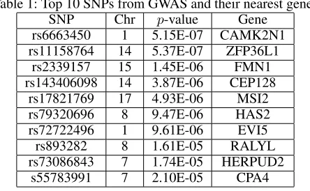
We present the Manhattan plot and the QQ plot of the GWAS results in Figure 5. The top 10 loci along with their

p-values are summarized in Table 1. As can be seen, no genome-wide significant marker(p-value <1.08×10−7₎

(6)

Figure 3: Histograms of wild bootstrap statistics for differ-ent MAF intervals with fixedλn = 10−2, along with their density approximations by mixed chis-quare distribution.

Figure 4: QQ Plots of wild bootstrap statistics for different MAF intervals for fixedλn = 10−2.

Figure 5: Visualization of GWAS results: Manhattan Plot and QQ Plot of the p-values of 450,899 SNPs.

ZFP36L1, CEP128, HAS2 and EVI5 are risk genes impli-cated by certain neurodegenerative diseases (Yuan et al. 2013; Perga et al. 2015; Mowry et al. 2013; Le-Niculescu et al. 2009). MSI2 gene is known to be related to the proliferation and maintenance of stem cells in the central nervous system (Sakakibara et al. 2001).

Conclusion

We proposed a powerful functional global testing framework (PFGT) to perform statistical inference on the varying coeffi-cient model. The asymptotic distribution of the test statistic has been systematically studied and we provided a strategy to adaptively select the optimal tuning parameter in order to maximize the testing power.

(7)

Table 1: Top 10 SNPs from GWAS and their nearest genes

SNP Chr p-value Gene

rs6663450 1 5.15E-07 CAMK2N1

rs11158764 14 5.37E-07 ZFP36L1

rs2339157 15 1.45E-06 FMN1

rs143406098 14 3.87E-06 CEP128

rs17821769 17 4.93E-06 MSI2

rs79320696 8 9.47E-06 HAS2

rs72722496 1 9.61E-06 EVI5

rs893282 8 1.61E-05 RALYL

rs73086843 7 1.74E-05 HERPUD2

s55783991 7 2.10E-05 CPA4

Acknowledgments

Dr. Zhu’s research was partially supported by the National Institutes of Health grants MH086633 and MH116527.

References

Cecchi, F., and Hegde, N. 2017. Adaptive active hypothesis testing under limited information. InAdvances in Neural Information Processing Systems, 4038–4046.

Fan, J., and Gijbels, I. 2018. Local polynomial modelling and its applications: monographs on statistics and applied probability, volume 66. Routledge.

Grenander, U., and Miller, M. I. 2007. Pattern Theory From Representation to Inference. Oxford University Press. Hall, P.; M¨uller, H. G.; and Wang, J. L. 2006. Properties of principal component methods for functional and longitudinal data analysis.The Annals of Statistics1493–1517.

Heller, R., and Heller, Y. 2016. Multivariate tests of as-sociation based on univariate tests. InAdvances in Neural Information Processing Systems, 208–216.

Huang, C.; Thompson, P.; Wang, Y.; Yu, Y.; Zhang, J.; Kong, D.; Colen, R. R.; Knickmeyer, R. C.; and Zhu, H. 2017. Fgwas: Functional genome wide association analysis. Neu-roImage159:107–121.

Jenkinson, M.; Beckmann, C. F.; Behrens, T. E.; Woolrich, M. W.; and Smith, S. M. 2012. Fsl.NeuroImage62(2):782– 790.

Jitkrittum, W.; Szab´o, Z.; Chwialkowski, K. P.; and Gretton, A. 2016. Interpretable distribution features with maximum testing power. InAdvances in Neural Information Processing Systems, 181–189.

Jitkrittum, W.; Xu, W.; Szab´o, Z.; Fukumizu, K.; and Gretton, A. 2017. A linear-time kernel goodness-of-fit test. In Ad-vances in Neural Information Processing Systems, 261–270. Kendall, D. G.; Barden, D.; Carne, T. K.; and Le, H. 2009.

Shape and shape theory, volume 500. John Wiley & Sons. Le-Niculescu, H.; Patel, S. D.; Bhat, M.; Kuczenski, R.; Faraone, S. V.; Tsuang, M. T.; McMahon, F. J.; Schork, N. J.; Nurnberger Jr, J. I.; and Niculescu Iii, A. B. 2009. Con-vergent functional genomics of genome-wide association data for bipolar disorder: Comprehensive identification of

candidate genes, pathways and mechanisms. American Jour-nal of Medical Genetics Part B: Neuropsychiatric Genetics

150(2):155–181.

Li, Y., and Hsing, T. 2010. Uniform convergence rates for nonparametric regression and principal component analy-sis in functional/longitudinal data. The Annals of Statistics

38(6):3321–3351.

Lisman, J.; Schulman, H.; and Cline, H. 2002. The molecular basis of camkii function in synaptic and behavioural memory.

Nature Reviews Neuroscience3(3):175.

Liu, J., and Coull, B. 2017. Robust hypothesis test for nonlinear effect with gaussian processes. In Advances in Neural Information Processing Systems, 795–803.

McMahon, M. A. B., and Thompson, P. M. 2017. Enhancing neuroimaging genetics through meta analysis: global collab-orations in psychiatry by the enigma consortium.European Neuropsychopharmacology27:S715.

Miller, M. I., and Qiu, A. 2009. The emerging discipline of computational functional anatomy.NeuroImage45:S16–S39. Mowry, E. M.; Carey, R. F.; Blasco, M. R.; Pelletier, J.; Du-quette, P.; Villoslada, P.; Malikova, I.; Roger, E.; Kinkel, R. P.; and McDonald, J. 2013. Multiple sclerosis susceptibility genes: associations with relapse severity and recovery. PloS one8(10):e75416.

Perga, S.; Montarolo, F.; Martire, S.; Berchialla, P.; Maluc-chi, S.; and Bertolotto, A. 2015. Anti-inflammatory genes associated with multiple sclerosis: a gene expression study.

Journal of neuroimmunology279:75–78.

Petersen, A., and M¨uller, H. G. 2016. Functional data analysis for density functions by transformation to a hilbert space.The Annals of Statistics44(1):183–218.

Qu, S., and Wang, X. 2017. Optimal global test for functional regression. arXiv preprint arXiv:1710.02269.

Sakakibara, S. I.; Nakamura, Y.; Satoh, H.; and Okano, H. 2001. Rna-binding protein musashi2: developmentally regu-lated expression in neural precursor cells and subpopulations of neurons in mammalian cns. Journal of Neuroscience

21(20):8091–8107.

Sen, R.; Suresh, A. T.; Shanmugam, K.; Dimakis, A. G.; and Shakkottai, S. 2017. Model-powered conditional indepen-dence test. InAdvances in Neural Information Processing Systems, 2955–2965.

Smith, S. M., and Nichols, T. E. 2009. Threshold-free cluster enhancement: addressing problems of smoothing, threshold dependence and localisation in cluster inference.NeuroImage

44:83–98.

Smith, S. M.; Jenkinson, M.; Johansen-Berg, H.; Rueckert, D.; Nichols, T. E.; Mackay, C. E.; Watkins, K. E.; Ciccarelli, O.; Cader, M. Z.; Matthews, P. M.; and Behrens, T. E. 2006. Tract-based spatial statistics: voxelwise analysis of multi-subject diffusion data. NeuroImage31:1487–1505.

Srivastava, A., and Klassen, E. P. 2016. Functional and shape data analysis. Springer.

(8)

Trevor, H.; Tibshirani, R.; and Friedman, J. H. 2009. The Elements of Statistical Learning: Data Mining, Inference, and Prediction (2nd). Hoboken, New Jersey.: Springer. Wang, X., and Ruppert, D. 2015. Optimal prediction in an additive functional model.Statistica Sinica567–589. Yuan, M., and Cai, T. T. 2010. A reproducing kernel hilbert space approach to functional linear regression. The Annals of Statistics38(6):3412–3444.

Yuan, Y.; Tang, B.; Yu, R.; Li, K.; Lv, Z.; Yan, X.; and Guo, J. 2013. Marginal association between snp rs2046571 of the has2 gene and parkinson’s disease in the chinese female population.Neuroscience letters552:58–61.