Continuous Acceptance Sampling plans for
Truncated Lindley Distribution Based on
CUSUM Schemes
S.Dhanunjaya1, Dr P. Mohammed Akhtar2, Dr. G.Venkatesulu3
1. Research scholar,Dept. of Statistics, Sri Krishanadevaraya University, Anantapuramu-515003,AP, INDIA 2. Professor, Dept. of Statistics, Sri Krishanadevaraya University, Anantapuramu-515003,AP, INDIA.
3. Asst. statistical officer, Tadipatri, Anantapuramu Dt., AP, INDIA.
ABSTRACT : This paper is on the study of continuous acceptance sampling plans for Truncated Lindley
distribution and optimization of CUSUM Schemes by using Gauss- Chebyshev integration method. In most of the life test experiments, the Truncated failure models are used to determine an optimal Truncated point. In the present study, we assume that the life of the units produced is distributed according to Truncated Lindley distribution. In a situation where there is a constraint on the lower part and upper part of the lifetime of units, Truncated failure models can be employed to study lifetime behavior of the items. Thus we study the lifetime of the units by using Truncated Lindley failure model. The objective of this paper is to optimize CASP – CUSUM Schemes through Truncated Lindley distribution. Solving integral equations by the Method of Gauss – Chebyshev integration we determine the probability of acceptance at various hypothetical values of the parameters. Finally based on the obtained results we determine the maximum values of Average Run Length and Probability of Acceptance.
Keywords: CASP – CUSUM Schemes, Optimal Truncated Point, optimal lower Truncated Point, Optimal upper
Truncated Point, Truncated Lindley distribution.
I. INTRODUCTION
In modern days consumers are sensitive with regard to the quality and reliability of the products. In ordered to meet consumer‟s satisfaction or demand, the manufacturer has to produce the items with high quality and reliability. Further, they have to make sure that the process should be free from assignable causes and eliminate assignable causes from the production process. For this statistical devices have been introduced by many researchers. In the beginning, Dodge and Roming introduced acceptance sampling plans for product control. Quality of the products is being maintained in two distinct phases namely 1. Process control 2. Product control. Maintaining the quality of the products by using quality control charts is called process control while maintaining the quality of the products by the sampling inspection method is called product control. As per as product control is concerned much research work has been carried out by Hawkins[4], verdeman[9] etc.
The acceptance sampling plan was first applied in the US military for testing the bullets during World War II. For instance, if every bullet tested in advance, no bullets are available for shipment, and on the other hand, if no bullets are tested, then disaster may occur in the battlefield at the crucial time. An acceptance sampling plan is a middle path between 100% inspection and no inspection.
An acceptance sampling plan is an essential device in Statistical Quality Control. In most of the statistical quality control experiments, it 100 % inspection of the items produced is not possible due to various reasons. For instance, 100% inspection involves, more time, more money, manpower, material, machinery etc. even the sample is finite, 100% inspection practically not feasible in case of explosive type materials like crackers, bombs, batteries, bulbs etc. The test can be performed without waiting until all the products fail, and then testing time can be reduced significantly. For the purpose of reduces test time and cost, obviously truncated life model is used.
Life tests experiments are carried out in order to obtain the lifetime of an item (i.e. time to its failure or the stops working satisfactorily). Sometimes, it may time consuming process as we have to wait until all the products fail in a life test if the lifetimes of products are high.
Hawkins, D. M. [4] Proposed a fast accurate approximation for ARL‟s of a CUSUM Control Charts. This approximation can be used to evaluate the ARL‟s for Specific parameter values and the out of control ARL‟s of location and scale CUSUM Charts.
Kakoty. S., Chakravarthy A.B. [6] Determined CASP-CUSUM charts under the assumption that the variable under study follows a Truncated Normal Distribution. Generally, truncated distributions are employed in many practical phenomena where there is a constraint on the lower and upper limits of the variable under study. For example, in the production engineering items, the sorting procedure eliminates items above or bellows designated tolerance limits. It is worthwhile to note that any continuous variable is first approximated as an exponential variable.
Vardeman.S, Di-ou Ray [9] was introduced CUSUM control charts under the restriction that the values are regard to quality is exponentially distributed. Further, the phenomena under study are the occurrence of the rate of rare events and the inter-arrival times for a homogenous poison process are identically independently distributed exponential random variables.
Lonnie. C. Vance [7], considered Average Run Length of Cumulative Sum Control Charts for controlling for normal means and to determine the parameters of a CUSUM Chart. To determine the parameters of the CUSUM Chart the acceptable and unacceptable quality levels along with the desired respective ARL's are considered.
Mohammed Akhtar. P and Sarma K.L.A.P [1] analyzed and Optimization of CASP-CUSUM Schemes based on truncated two parametric Gamma distribution and evaluate L (0), L' (0) and the probability of Acceptance and also Optimized CASP-CUSUM Schemes based numerical results.
Narayana Murthy, B.R. and Mohammed Akhtar.P[10] proposed an Optimization of CASP CUSUM Schemes based on Truncated Log-logistic distribution and evaluate the probability of acceptance for different parameter values.
Sainath.B and Mohammed Akhtar .P [12] studied an Optimization of CASP-CUSUM Schemes based on truncated Burr distribution and the results were analyzed at different values of the parameters.
Venkatesulu.G and Mohammed Akhtar.P[13] Determined Truncated Gompertz Distribution and its Optimization of CASP-CUSUM Schemes by changing the values of the parameters and finally, critical comparisons are drawn based on the obtained numerical results.
Venkatesulu.G and Mohammed Akhtar.P[17] Determined Continuous Acceptance Sampling Plans for Truncated Lomax Distribution Based on CUSUM schemes by changing the values of the parameters and finally, critical comparisons are drawn based on the obtained numerical results.
In the present paper, it is determined type-C OC Curves of CASP-CUSUM Schemes when the variable under study follows truncated Lindley Distribution. Thus it is more worthwhile to study some interesting characteristics of Type-C OC Curves based on this distribution.
II. LINDLEY DISTRIBUTION
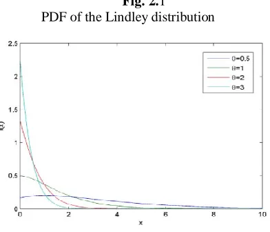
A continuous random variable X assuming non-negative values is said to have Lindley distribution with parameters θ > 0 and its probability density function is given by
𝑓 𝑥 = 𝜃
2
𝜃 +1(1 + 𝑥) 𝑒
−𝜃𝑥 ; 𝑥 > 0, 𝜃 > 0 ……. (2.1)
Lindley distribution is the mixture of the exponential (θ) and gamma (2, θ) distribution with pdfs f(x) = θ𝑒−𝜃𝑥 and f(x) = 𝜃2𝑥𝑒−𝜃𝑥 respectively. Also, the mixing proportions are 𝜃
1 +𝜃 and 1
In the lifetime theory, we study the life of a system or an item. The word system (or item or component) is defined as an arbitrary device performing its intended task. A system can be an electrical, electronic, mechanical or chemical device. Apart from manmade systems such as human beings, plants, animals, etc. that are included in the lifetime analysis.
A lifetime distribution represents an attempt to describe, mathematically, the length of the life of a system or device, with the advancement in technology new and complex types of consumable items are being produced every day. To model the failure data of such types of new devices we need more possible statistical distributions to be considered as lifetime models.
The Lindley distribution was first proposed by Lindley[15]in connection with the fiducial distribution was also compounded with Poisson distribution, by shankaran[16]. In a recent study, Ghitany et.al.[14] have discussed Lindley distribution in detail with its applications and real data example. In reliability studies, a sample of n items is put on the test and the experiment is terminated when all of them fail. This procedure may take a long time when the lifetime distribution of items has a thick tail. Moreover, if the items are expensive such as medical equipment‟s, it is costly to gather the whole sample information. There are many situations where experimental units are lost or removed from the test, before the complete failure.
In view of the above, truncation is used in life testing to save time and cost testing units. The removal of units in a test may be pre-planned. Data obtained from such experiments are called Truncated sample. Life data are collected for estimating the parameters and reliability functions when complete sample information is not available, we use the information that “the Truncated experimental units –did not fail up to a specific time” in the estimation procedure.
PDF of the Lindley distribution graph is given by
Fig. 2.1
PDF of the Lindley distribution
A. Truncated Lindley Distribution
It is the ratio of the probability density function of the Lindley distribution to their corresponding cumulate distribution function at point B.
The random variable X is said to follow a truncated Lindley Distribution as
f
B(X) =
𝜃 2
𝜃 +1(1+𝑥) 𝑒−𝜃𝑥
1−𝜃 +1+𝜃𝐵𝜃 +1 𝑒−𝜃𝐵, θ>0,x>0 ……….(2.2)
A new distribution with one parameters named a Truncated Lindley distribution is proposed which is more flexible than many well-known heavily tailed distributions. The importance of Truncated Lindley distribution is illustrated by means of the two real datasets is evaluated. The results indicate that the new distribution can provide better fits than Exponential, Weibull, Gamma, Log-normal, Log-logistic and generalized extreme value distribution in insurance. Therefore, Truncated Lindley distribution can be an alternative for modeling the catastrophe loss in insurance applications.
III. DESCRIPTION OF THE PLAN AND TYPE- C OC CURVE
Battie [2] has suggested the method for constructing continuous acceptance sampling plans. The procedure, suggested by him consists of a chosen decision interval namely, “Return interval” with the length h‟,
above the decision line is taken. We plot on the chart the sum
S
m
(
X
i
k
1)
X
i'
s
(
i
1
,
2
,
3
...)
are distributed independently and k1 is the reference value. If the sum lies in the area of the normal chart, the product is accepted and if it lies on the return chart, then the product is rejected, subject to the following assumptions.1. When the recently plotted point on the chart touches the decision line, then the next point to be plotted at the maximum, i.e., h+h‟.
2. When the decision line is reached or crossed from above, the next point on the chart is to be plotted from the baseline.
When the CUSUM falls in the return chart, network or a change of specification may be employed rather than outright rejection.
The procedure, in brief, is given below. 1. Start plotting the CUSUM at 0.
2. The product is accepted
S
m
(
X
i
k
)
h
;
when Sm< 0, return cumulative to 0.3. When h <Sm<h+h‟ the product is rejected: when Sm crossed h, i.e., when Sm>h+h‟ and continue rejecting product until Sm>h+h‟ return cumulative to h+h‟.
The Type-C, OC function, which is defined as the probability of acceptance of an item as a function of incoming quality, when the sampling rate is the same in acceptance and rejection regions. Then the probability of acceptance P (A) is given by
)
0
(
'
)
0
(
)
0
(
)
(
L
L
L
A
P
…… (3.1)Where L (0) = Average Run Length in acceptance zone and L‟ (0) = Average Run Length in rejection zone.
Page E.S. [8] has introduced the formulae for L (0) and L‟ (0) as
1
(
0
)
)
0
(
)
0
(
P
N
L
…… (3.2)
)
0
(
'
1
)
0
(
'
)
0
(
'
P
N
L
…… (3.3)Where P (0) =Probability for the test starting from zero on the normal chart, N (0) = ASN for the test starting from zero on the normal chart, P‟ (0) = Probability for the test on the return chart and
N‟ (0) = ASN for the test on the return chart
He further obtained integral equations for the quantities P (0), N (0), P‟ (0), N‟ (0) as follows
F
k
z
hP
y
f
y
k
z
dy
z
P
0
1
1
)
(
)
(
)
(
)
(
, ... (3.4)
hN
y
f
y
k
z
dy
z
N
0
1
)
(
)
(
1
)
B z k hdy
z
k
y
f
y
P
dy
y
f
z
P
1 0 1)
(
)
(
'
)
(
)
(
'
.….. (3.6),
)
(
)
(
'
1
)
(
'
1 0dy
z
k
y
f
y
N
z
N
h
…… (3.7)
h Adx
x
f
x
F
(
)
1
(
)
:
dy
y
f
z
k
F
z k A
)
1
1(
)
(
1and z is the distance of the starting of the test in the normal chart from zero.
IV. METHOD OF SOLUTION
We first express the integral equation (3.4) in the form
d cdt
t
F
t
x
R
X
Q
X
F
(
)
(
)
(
,
)
(
)
…… (4.1)Where
)
(
)
,
(
),
(
)
(
),
(
)
(
z
k
y
f
t
X
R
z
k
F
X
Q
z
P
X
F
Let the integral
d
c
dx
x
f
I
(
)
be transformed to. . …. (4.2)
Where c d d c x y
2 ( )ai‟s and ti‟s respectively the weight factor and abscissa for the Gauss-Chebyshev
polynomial, given in Jain M.K. and et al [4] using (4.1) and (4.2),(3.4) can be written as
..…. (4.3)
Since equation (4.3) should be valid for all values of x in the interval (c, d), it must be true for x=ti, i = 0 to n then obtain.
….. (4.4) J=0 to n
Substituting
),
4
.
4
(
,
)
(
0
,
)
(
,
)
(
t
F
Q
t
Q
i
to
n
in
F
i
i i
i
we get)] ) , ( . ... ) , ( ) , ( [
2 0 0 0 0 1 0 1 1 0
0
0 a R t t F aR t t F anR t tn Fn
c d Q
F
)
(
2
)
(
2
i id c
t
f
a
c
d
dy
y
f
c
d
I
)
(
)
,
(
2
)
(
)
(
a
iR
x
t
iF
t
ic
d
X
Q
X
F
)
(
)
,
(
2
)
(
)
(
t
iQ
t
id
c
a
iR
t
jt
iF
t
i)] ) , ( . ... ) , ( ) , ( [
2 0 1 0 0 1 1 1 1 1
1
1 a R t t F aR t t F anR t tn Fn
c d Q
F
………… ………… ……….. ……… ………… …………. ……….. ………. )] ) , ( . ... ) , ( ) , ( [
2 0 n 0 0 1 n 1 1 n n n n
n
n a R t t F a R t t F a R t t F
c d Q
F …… (4.5)
In the system of equations except for Fi, i= 0,1,2………n are known and hence can be solved for Fi, we solved the system of equations by the method of Iteration. For this, we write the system (4.5) as
)]
)
,
(
...
)
,
(
)
,
(
[
)]
,
(
1
[
Ta
0R
t
0t
0F
0
Q
0
T
a
0R
t
0t
0F
0
a
1R
t
0t
1F
1
a
nR
t
0t
nF
n)]
)
,
(
...
)
,
(
)
,
(
[
)]
,
(
1
[
Ta
1R
t
1t
1F
1
Q
1
T
a
0R
t
1t
0F
0
a
1R
t
1t
1F
1
a
nR
t
1t
nF
n………. ………. ………….. ………… ………. ……….. ..………… …………
)]
)
,
(
...
)
,
(
)
,
(
[
)]
,
(
1
[
Ta
nR
t
nt
nF
n
Q
n
T
a
0R
t
nt
0F
0
a
1R
t
nt
1F
1
a
nR
t
nt
nF
n .. (4.6)Where
2
c d T
To start the Iteration process, let us put
F
1
F
2
....
F
n
0
in the first equation of (3.6), we thenobtain a rough value of
F
0. Putting this value ofF
0 andF
1
F
2
....
F
n
0
on the second equation, we getthe rough valueF1 and so on. This gives the first set of values
F
i= 0,1,2,...,n which are just the refined values ofi
F
= 0,1,2,…,n. The process is continued until two consecutive sets of values are obtained up to a certain degree of accuracy. In a similar way solutions P(0), P‟ (0), N (0) and N‟ (0) can be obtained.V. COMPUTATION OF ARL’s AND P (A)
TABLE – 5.1 TABLE – 5.2
Values of ARL‟s and TYPE – C OC curves when Values of ARL‟s and TYPE –C OC curves when
k=1, 𝜃 = 0.5, h=0.10, h‟ = 0.10 k=1, 𝜃 = 0.5, h=0.12, h‟ = 0.12
B L(0) L’(0) P(A)
1.5 3.02319 1.1241715 0.7289429 1.4 3.57124 1.1351991 0.7587990 1.3 4.53633 1.1484455 0.7979789 1.2 6.67966 1.1646085 0.8515338 1.1 15.48778 1.1847011 0.9289427
B L(0) L’(0) P(A)
TABLE – 5.3 TABLE – 5.4
Values of ARL‟s and TYPE – C OC curves when Values of ARL‟s and TYPE –C OC curves when
k=1, 𝜃 = 0.5, h=0.15, h‟ = 0.15 k=1, 𝜃 = 0.5, h=0.18, h‟ = 0.18
TABLE – 5.5 TABLE – 5.6
Values of ARL‟s and TYPE – C OC curves when Values of ARL‟s and TYPE –C OC curves when
k=1, 𝜃 = 1, h=0.10, h‟ = 0.10 k=1, 𝜃 = 1, h=0.12, h‟ = 0.12
B L(0) L’(0) P(A)
1.5 3.75474 1.1321192 0.7683339 1.4 4.45785 1.1405776 0.7962682 1.3 5.73442 1.1507558 0.8328648 1.2 8.7489 1.1631787 0.8826514 1.1 24.41226 1.1786009 0.9539444
TABLE – 5.7 TABLE – 5.8
Values of ARL‟s and TYPE – C OC curves when Values of ARL‟s and TYPE –C OC curves when
k=1, 𝜃= 1, h=0.15, h‟ = 0.15 k=1, 𝜃= 1, h=0.18, h‟ = 0.18
B L(0) L’(0) P(A)
1.5 3.77081 1.2020680 0.7582753 1.4 4.53356 1.2151002 0.7886289 1.3 5.97544 1.2307678 0.8292072 1.2 9.70186 1.2498605 0.8858754 1.1 41.12255 1.2734979 0.9699619
TABLE – 5.9 TABLE – 5.10
Values of ARL‟s and TYPE – C OC curves when Values of ARL‟s and TYPE –C OC curves when
k=1, 𝜃= 1.5, h=0.10, h‟ = 0.10 k=1, 𝜃= 1.5, h=0.12, h‟ = 0.12
B L(0) L’(0) P(A)
1.5 3.09465 1.1911361 0.7220730 1.4 3.69184 1.2084924 0.7533858 1.3 4.77500 1.294028 0.7967451 1.2 7.33418 1.2549989 0.8538861 1.1 20.72701 1.2869266 0.9415404
B L(0) L’(0) P(A)
1.5 3.14317 1.2327865 0.7182821 1.4 3.77406 1.2541620 0.7505755 1.3 4.94052 1.2799416 0.7942368 1.2 7.81495 1.3115269 0.8562942 1.1 26.20148 1.350948 0.9509681
B L(0) L’(0) P(A)
1.5 3.75892 1.1598797 0.7641948 1.4 4.48498 1.1701622 0.7930799 1.3 5.82453 1.1825358 0.8312366 1.2 9.10058 1.1976364 0.8837045 1.1 29.14358 1.2163759 0.9599348
B L(0) L’(0) P(A)
1.5 3.78960 1.2446542 0.7527629 1.4 4.59221 1.2603865 0.7846450 1.3 6.14763 1.2792554 0.8277534 1.2 10.41283 1.3021698 0.8888459 1.1 69.95697 1.3303918 0.9813376
B L(0) L’(0) P(A)
1.5 4.12908 1.149316 0.7822580 1.4 4.89669 1.1558272 0.8090336 1.3 6.33187 1.167169 0.8447465 1.2 9.92030 1.1734143 0.8942271 1.1 34.17790 1.1855054 0.9664765
B L(0) L’(0) P(A)
TABLE – 5.11 TABLE – 5.12
Values of ARL‟s and TYPE – C OC curves when Values of ARL‟s and TYPE –C OC curves when
k=1, 𝜃= 1.5, h=0.15, h‟ = 0.15 k=1, 𝜃= 1.5, h=0.18, h‟ = 0.18
TABLE – 5.13 TABLE – 5.14
Values of ARL‟s and TYPE – C OC curves when Values of ARL‟s and TYPE –C OC curves when
k=2, 𝜃= 0.5, h=0.10, h‟ = 0.10 k=2, 𝜃= 0.5, h=0.12, h‟ = 0.12
TABLE – 5.15 TABLE – 5.16
Values of ARL‟s and TYPE – C OC curves when Values of ARL‟s and TYPE –C OC curves when
k=2, 𝜃= 0.5, h=0.15, h‟ = 0.15 k=2, 𝜃= 0.5, h=0.18, h‟ = 0.18
B L(0) L’(0) P(A)
1.5 3.72079 1.2655942 0.7461901 1.4 4.49168 1.2762661 0.7787312 1.3 6.01939 1.2890307 0.8236238 1.2 10.41075 1.3043975 0.8886572 1.1 127.10031 1.3230114 0.9896981
B L(0) L’(0) P(A)
1.5 3.84850 1.2235893 0.7587605 1.4 4.61607 1.2329966 0.7891976 1.3 6.10639 1.2443477 0.8307180 1.2 10.17729 1.2581762 0.8899760 1.1 62.91886 1.2752082 0.9801351
B L(0) L’(0) P(A)
2.5 5.54769 1.0704013 0.8382614 2.4 6.68904 1.0733435 0.8617250 2.3 8.64817 1.076094 0.8892921 2.2 12.78743 1.0802507 0.9221030 2.1 27.27292 1.0843309 0.9617618
B L(0) L’(0) P(A)
2.5 5.58003 1.0850230 0.8372070 2.4 6.74212 1.0885978 0.8609837 2.3 8.74869 1.0925672 0.8889809 2.2 13.03798 1.0969955 0.9223914 2.1 28.60192 1.1019602 0.9629018
B L(0) L’(0) P(A)
2.5 5.68440 1.1299587 0.8341798 2.4 6.91345 1.1355158 0.8589240 2.3 9.07523 1.1416944 0.8882545 2.2 13.87187 1.1485962 0.9235312 2.1 33.57642 1.1563451 0.9667073
B L(0) L’(0) P(A)
TABLE – 5.17 TABLE – 5.18
Values of ARL‟s and TYPE – C OC curves when Values of ARL‟s and TYPE –C OC curves when
k=3, 𝜃= 0.5, h=0.10, h‟ = 0.10 k=3, 𝜃= 0.5, h=0.12, h‟ = 0.12
B L(0) L’(0) P(A)
3.5 9.18166 1.0519872 0.8972031 3.4 11.18532 1.0532259 0.9139419 3.3 14.61046 1.0545619 0.9326804 3.2 21.79135 1.0560050 0.9537800 3.1 46.35325 1.0575676 0.9776936
TABLE-5.19 TABLE – 5.20
Values of ARL‟s and TYPE – C OC curves when Values of ARL‟s and TYPE –C OC curves when
k=3, 𝜃= 0.5, h=0.15, h‟ = 0.15 k=3, 𝜃= 0.5, h=0.18, h‟ = 0.18
TABLE – 5.21 TABLE – 5.22
Values of ARL‟s and TYPE – C OC curves when Values of ARL‟s and TYPE –C OC curves when
k=3, 𝜃= 1, h=0.10, h‟ = 0.10 k=3, 𝜃= 1, h=0.12, h‟ = 0.12
TABLE – 5.23 TABLE – 5.24
Values of ARL‟s and TYPE – C OC curves when Values of ARL‟s and TYPE –C OC curves when
k=3, 𝜃= 1, h=0.15, h‟ = 0.15 k=3, 𝜃= 1, h=0.18, h‟ = 0.18
B L(0) L’(0) P(A)
3.5 9.23409 1.0626869 0.8967941 3.4 11.26990 1.0641876 0.9137198 3.3 14.76772 1.0658062 0.9326867 3.2 22.17447 1.0675551 0.9540679 3.1 48.28651 1.0694492 0.9783319
B L(0) L’(0) P(A)
3.5 9.31535 1.0789251 0.8962001 3.4 11.40117 1.0808274 0.9134091 3.3 15.01297 1.0828794 0.9327230 3.2 22.78028 1.0850977 0.9545326 3.1 51.52607 1.0875008 0.9793304
B L(0) L’(0) P(A)
3.5 9.39989 1.0953890 0.8956303 3.4 11.53797 1.0977030 0.9131267 3.3 15.27012 1.1002001 0.9327930 3.2 23.42673 1.1029000 0.9550380 3.1 55.25562 1.1058261 0.9803798
B L(0) L’(0) P(A)
3.6 23.70767 1.0954925 0.9558325 3.5 28.86360 1.0963101 0.9634075 3.4 37.92297 1.0972096 0.9718810 3.3 57.90563 1.0981998 0.9813877 3.2 137.85223 1.0992916 0.9920887
B L(0) L’(0) P(A)
3.6 22.81950 1.0791016 0.9548467 3.5 27.46539 1.0797759 0.9621730 3.4 35.37530 1.0805175 0.9703609 3.3 51.76255 1.0813341 0.9795372 3.2 105.58409 1.0822343 0.989540
T L(0) L’(0) P(A)
3.6 26.87087 1.145076 0.9591095 3.5 34.09224 1.1468668 0.9674547 3.4 48.37973 1.1482517 0.9768161 3.3 38.75285 1.1497766 0.9873515 3.2 1538.61462 1.1514577 0.9992522
T L(0) L’(0) P(A)
TABLE – 5.25 TABLE – 5.26
Values of ARL‟s and TYPE – C OC curves when Values of ARL‟s and TYPE –C OC curves when
k=3, 𝜃= 1.5, h=0.10, h‟ = 0.10 k=3, 𝜃= 1.5, h=0.12, h‟ = 0.12
B L(0) L’(0) P(A)
4.2 138.87761 1.1124036 0.9920537 4.1 168.65768 1.1125373 0.9934468 4.0 223.35858 1.1126899 0.9950430 3.9 354.76886 1.1128641 0.9968730 3.8 1081.21545 1.1130632 0.9989716
TABLE – 5.27 TABLE – 5.28
Values of ARL‟s and TYPE – C OC curves when Values of ARL‟s and TYPE –C OC curves when
k=3, 𝜃= 1.5, h=0.15, h‟ = 0.15 k=3, 𝜃= 1.5, h=0.18, h‟ = 0.18
TABLE – 5.29 TABLE – 5.30
Values of ARL‟s and TYPE – C OC curves when Values of ARL‟s and TYPE –C OC curves when
k=4, 𝜃= 0.5, h=0.10, h‟ = 0.10 k=4, 𝜃= 0.5, h=0.12, h‟ = 0.12
B L(0) L’(0) P(A)
4.5 14.54626 1.0433494 0.9330741 4.4 17.83912 1.0439847 0.9447135 4.3 23.47789 1.0446600 0.9574000 4.2 35.34037 1.0453786 0.9712695 4.1 76.34338 1.0461441 0.9864821
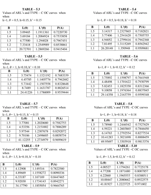
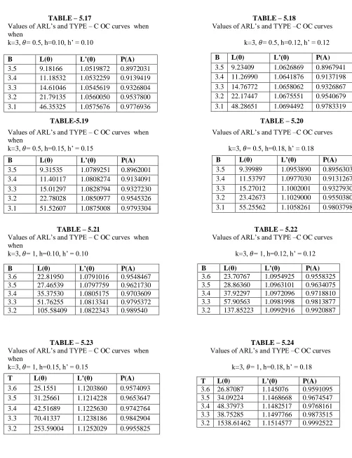
VI. NUMERICAL RESULTS AND CONCLUSIONS
At the hypothetical values of the parameters, 𝜃, k, h and h‟ are given at the top of each table, we determine optimum truncated point B at which P (A) the probability of accepting an item is maximum and also obtained ARL's values which represent the acceptance zone L(0) and rejection zone L'(0) values. The values of truncated point B of random variable X, L(0), L'(0) and the values for Type-C Curve, i.e. P (A) are given in columns I, II, III, and IV respectively.
From the above tables 5.1 to 5.30 we made the following conclusions
1. From the Table 5.1to 5.30, it is observed that the values of P (A) are increased as the value of truncated point decreases thus the Truncated point of the random variable and the various parameters for CASP-CUSUM are related.
B L(0) L‟(0) P(A) 4.4 166.88481 1.1349635 0.9932451 4.3 201.33347 1.1350864 0.99439938 4.2 263.45517 1.1352270 0.9957095 4.1 406.84796 1.1353873 0.9972171 4.0 1075.17676 1.1355705 0.9989449
B L(0) L’(0) P(A)
4.7 274.26886 1.1685587 0.957575 4.6 343.62500 1.1686609 0.9966105 4.5 483.28925 1.1687777 0.9975874 4.4 902.44604 1.1689112 0.9987064
4.3 98418.44531 1.1690637 0.9999881
B L(0) L’(0) P(A)
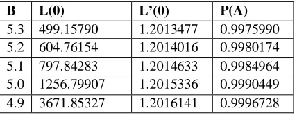
5.3 499.15790 1.2013477 0.9975990 5.2 604.76154 1.2014016 0.9980174 5.1 797.84283 1.2014633 0.9984964 5.0 1256.79907 1.2015336 0.9990449 4.9 3671.85327 1.2016141 0.9996728
B L(0) L’(0) P(A)
4.5 14.64451 1.0522320 .9329649 4.4 17.99573 1.0530005 0.9447207
4.3 23.76588 1.0538173 0.9575411
4.2 36.03692 1.0546868 0.9715654
2. From Table 5.1 to 5.30we observe that it can be maximized the Truncated point B by increasing the value of k.
3. From Table 5.1 to 5.30, it is observed that at the maximum level of probability of acceptance P (A) the Truncated point B from 5.1to 1.1 as the value of h changes from 0.10 to 0.18.
4. From the Table 5.1 to 5.30, it was observed that the value of L (0) and P (A) is increased as the value of Truncated point decreases thus the Truncated point of the random variable and the various parameters for CASP-CUSUM are related.
5. From Table 5.1 to 5.30, it was observed that the Truncated point B changes from 3.0 to 1.1 and P (A) are as
15
.
0
h
maximum i.e. 0.9999881. Thus truncated point B and h are inversely related and hand P (A) are positively related.6. From Table 5.1 to 5.30 it is observed that the optimal Truncated point changes from 1.1 to 4.3 as
15
.
0
h
.7. It is observed that the Table -6.1 values of Maximum Probabilities increased as the increased values of „k‟
as shown below the Figure-6.1.
8. It is observed that the Table-6.2 values of Maximum Probabilities increased as the values of h and h‟ as shown below the Figure-6.2
TABLE-6.2 θ = 0.5, B=3.1, k=3
h and h' P(A)
0.1 0.97769 0.12 0.97833 0.15 0.97933
0.18 0.98038
9. The various relations exhibited among the ARL's and Type-C OC Curves with the parameters of the CASP-CUSUM based on the above table 5.1 to 5.30 are observed from the following Table.
0.977 0.978 0.979 0.98 0.981
0 0.1 0.2
Figure-6.1
P(A)
0.977 0.978 0.979 0.98 0.981
0 0.1 0.2
Figure-6.2
P(A)
TABLE-6.1 θ = 0.5, h =0.10, h’=0.10
k P(A)
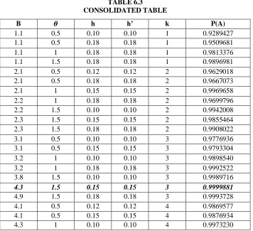
TABLE 6.3
CONSOLIDATED TABLE
By observing the Table- 6.3, we can conclude that the optimum CASP-CUSUM Schemes which have the values of ARL and P (A) reach their maximum i.e., 98418, 0.9999881 respectively, is
15
.
0
'
15
.
0
3
5
.
1
3
.
4
h
h
k
B
REFERENCES
[1] Akhtar, P. Md. and Sarma, K.L.A.P. (2004). “Optimization of CASP-CUSUM Schemes based on Truncated Gamma Distribution”. Bulletin of Pure and applied sciences, Vol-23E (No.2), pp215-223.
[2] Beattie, B.W. (1962). “A Continuous Acceptance Sampling procedure based upon a Cumulative Sums Chart for a number of defective”. Applied Statistics, Vol. 11(No.2), pp137- 147.
[3] Murphy, E.M., D.N.Nagpur (1972), “A Gompertz fit that fits: application to Canadian fertility patterns”, Demography, 9, pp35-50. [4] Hawkins, D.M. (1992). “A Fast Accurate Approximation for Average Lengths of CUSUM Control Charts". Journal of Quality
Technology, Vol. 24(No.1), pp37-43.
[5] Jain, M.K., Iyengar, S.R.K. and Jain, R.K. “Numerical Methods of Scientific and Engineering Computations”, Willy Eastern Ltd., New Delhi.
[6] Kakoty, S and Chakravaborthy, A.B., (1990), “A Continuous Acceptance Sampling Plan for Truncated Normal distribution based on Cumulative Sums”, Journal of National Institution for Quality and Reliability, Vol.2 (No.1), pp15-18.
[7] Lonnie, C. Vance. (1986). “Average Run Length of CUSUM Charts for Controlling Normal means”. Journal of Quality Technology, Vol.18, pp189-193.
[8] Page, E.S., (1954) “Continuous Inspection Schemes”, Biometrika, Vol. XLI, pp104- 114.
[9] Vardeman, S. And Di-ou Ray. (1985). “Average Run Length for CUSUM schemes Where observations are Exponentially Distributed”, Technometrics, vol. 27 (No.2), pp145- 150.
B 𝜽 h h’ k P(A)
1.1 0.5 0.10 0.10 1 0.9289427
1.1 0.5 0.18 0.18 1 0.9509681
1.1 1 0.18 0.18 1 0.9813376
1.1 1.5 0.18 0.18 1 0.9896981
2.1 0.5 0.12 0.12 2 0.9629018
2.1 0.5 0.18 0.18 2 0.9667073
2.1 1 0.15 0.15 2 0.9969658
2.2 1 0.18 0.18 2 0.9699796
2.2 1.5 0.10 0.10 2 0.9942008
2.3 1.5 0.15 0.15 2 0.9855464
2.3 1.5 0.18 0.18 2 0.9908022
3.1 0.5 0.10 0.10 3 0.9776936
3.1 0.5 0.15 0.15 3 0.9793304
3.2 1 0.10 0.10 3 0.9898540
3.2 1 0.18 0.18 3 0.9992522
3.8 1.5 0.10 0.10 3 0.9989716
4.3 1.5 0.15 0.15 3 0.9999881
4.9 1.5 0.18 0.18 3 0.9993728
4.1 0.5 0.12 0.12 4 0.9869577
4.1 0.5 0.15 0.15 4 0.9876934
[10] Narayana Muthy, B. R, Akhtar, P. Md and Venkataramudu, B.(2012) “Optimization of CASP-CUSUM Schemes based on Truncated Log-Logistic Distribution”. Bulletin of PureAnd Applied Sciences, Vol-31E (Math&Stat.): Issue (No.2), pp243-255.
[11] Narayana Muthy, B. R, Akhtar, P. Md and Venkataramudu, B. (2013) “Optimization of CASP-CUSUM Schemes based on Truncated Rayleigh Distribution”. International Journal of Engineering and Development, Volum 6, Issue 2, pp37-44.
[12] M.E Ghitany,B.Atieh,S.Nadarajah.(2008) “Lindley Distribution and its applications”. Mathematics and computers in simulation 78(2008) 493-506.
[13] B.Sainath, P.Mohammed Akhtar, G.Venkatesulu, and Narayana Muthy, B. R, (2016) “CASPCUSUM Schemes based on Truncated Burr Distribution using Lobatto Integration method, IOSR Journal of Mathematics (IOSR-JM), Vol-12, Issue 2, pp54-63.
[14] G.Venkatesulu, P.Mohammed Akhtar, B.Sainath and Narayana Murthy, B.R. (2017)“Truncated Gompertz Distribution and its Optimization of CASP- CUSUMSchemes”.Journal of Research in Applied Mathematics, Vol3-Issue7, pp19-28.
[15] D. V. Lindley, Fiducial distributions and Bayes'theorem. Journal of theRoyal Society, series B, 20 (1958), 102-107. [16] M. Sankaran, The discrete Poisson-Lindley distribution. Biometrics, 26(1970), 145-149.