Landscape Ecology vol. 9 no. 1 pp 47-57 (1994) SPB Academic Publishing bv, The Hague
Resolution and predictability: An approach to the scaling problem
Robert Costanza and Thomas Maxwell
Maryland International Institute for Ecological Economics, Center for Environmental and Estuarine Studies, University of Maryland, Box 38, Solomons, MD 20688-0038, USA
Keywords: Scaling, predictability, resolution, GIs, fractals, landscape modeling
Abstract
We analyzed the relationship between resolution and predictability and found that while increasing resolution provides more descriptive information about the patterns in data, it also increases the difficulty of accurately modeling those patterns. There are limits to the predictability of natural phenomenon at particular resolu- tions, and "fractal-like" rules determine how both "data" and "model" predictability change with reso- lution.
We analyzed land use data by resampling map data sets at several different spatial resolutions and measur- ing predictability at each. Spatial auto-predictability (Pa) is the reduction in uncertainty about the state of a pixel in a scene given knowledge of the state of adjacent pixels in that scene, and spatial cross-predictability (PC) is the reduction in uncertainty about the state of a pixel in a scene given knowledge of the state of cor- responding pixels in other scenes. Pa is a measure of the internal pattern in the data while PC is a measure of the ability of some other "model" to represent that pattern.
We found a strong linear relationship between the log of Pa and the log of resolution (measured as the number of pixels per square kilometer). This fractal-like characteristic of "self-similarity" with decreasing resolution implies that predictability may be best described using a unitless dimension that summarizes how it changes with resolution. While Pa generally increases with increasing resolution (because more informa- tion is being included), PC generally falls or remains stable (because it is easier to model aggregate results than fine grain ones). Thus one can define an "optimal" resolution for a particular modeling problem that balances the benefit in terms of increasing data predictability (Pa) as one'increases resolution, with the cost of decreasing model predictability (PC).
Introduction
We hypothesized that an important determinant of the predictability of phenomenon is the scale (reso- lution and extent) of the analysis. By resolution we mean "grain size" or the size of the smallest unit of measure, with increasing resolution corresponding to fine grain. We can distinguish at least two ways that resolution might affect predictability. One is the increasing difficulty of building predictive
models at increasingly finer resolution. For exam- ple, the position and velocity of individual mole- cules in a gas is highly unpredictable, but the tem- perature of the gas (which is an average of these motions at a much cruder resolution) is highly pre- dictable. Likewise, it is easier to predict general climate patterns than it is to predict the exact geographic location and timing of rainstorms (the weather).
48
detail to be observed and internal patterns in the data to be seen that may not have been observed at cruder resolutions. One example is the warm core gyres that form in the Gulf Stream that were not ob- served until remote sensing images including the proper thermal bands and of sufficiently fine reso- lution were available. Another example is the quest by the military to obtain high enough resolution satellite images to see the features (such as tanks and airplanes) of interest to them that would not appear on lower resolution images.
Some phenomenon are known to vary in a regu- lar way with resolution. For example, the regular relationship between the measured length of a coastline and the resolution at which it is measured is a fundamental one behind the concept of fractals (Mandelbrot 1977) and can be summarized in the following equation:
L = k s(1-D) (1)
where:
L = the length of the coastline or other “fractal” boundary
s = the size of the fundamental unit of measure or the resolution of the measurement
k = a scaling constant D = the fractal dimension
This convenient “scaling rule” has proved to be very useful in describing many kinds of complex boundaries and behaviors (Mandelbrot 1983, Milne
1988, Turner et al. 1987, 1989, Olsen and Schaffer
1990, Sugihara and May 1990). We hypothesized
that this same kind of relationship might exist be- tween resolution and predictability (and possibly other measures as well) and might be useful for developing scaling rules for understanding and modeling. We tested this hypothesis by calculating both data and model predictability for a number of landscapes at a number of different resolutions.
Measurement of predictability
Colwell (1 974) applied information theoretic con- cepts to the problem of estimating the degree of predictability of periodic phenomena. The method
is similar to autocorrelation analysis except that it is applicable to both interval and categorical data and may thus be more appropriate, for example, for comparing patterns of land cover. Predictabili- ty in this context refers to the reduction in uncer- tainty about one variable that can be gained by knowledge of another. For example, if the seasonal rainfall pattern in an area is predictable (e.g., there is always a severe dry summer), then knowing the time of year provides information about rainfall (if it’s summer, it must be dry). If there is no relation- ship between rainfall and season, time of year tells us little and the rainfall is relatively unpredictable from a knowledge of time of year.
These techniques can also be applied to spatial data (Turner et al. 1989). In this application, one is interested in the degree to which the uncertainty about the category of a particular pixel is reduced from knowledge of other aspects of the same scene, or from knowledge of aspects of other, related scenes. There are several aspects of a scene that might be used as predictors. We discuss two im- plementations based on (1) the state of adjacent pixels in the same scene (“auto-predictability” or
Pa); and (2) the state of corresponding pixels in
other, related scenes (“cross predictability” or PJ.
Other combinations of these two and higher level analyses ( i e . , adjacent pixel pairs, triplets, etc., or multiple cross comparisons) are also possible and useful for various purposes (Turner et al. 1989).
The method in general can determine if there are regularities in a spatial data set, ranked on a scale from 0 (totally unpredictable) to 1 (totally predict- able), and the answer can be interpreted as the degree of departure of the scene or comparison be- tween scenes from a random (totally unpredictable) pattern.
49
top of the matrix lying adjacent to the category listed along the left. This yields information about how predictable the patterns of adjacency are in the sample map data.
The contingency matrix can be any set of meaningful spatial relationships in the data. For example, another way of setting up the matrix is to define the predictability of one scene given another scene. For example, we might want to know the predictability of a landscape in one year given in- formation in some previous year@), or we might want to know the predictability of a real landscape compared to a landscape model’s output. We call this the “cross” predictability, because it provides information on the predictability of a given pixel’s category given knowledge of the category of the corresponding pixel in another scene.
Following Colwell(l974) we define Nij to be the elements in the contingency matrix (i.e., the num- ber of times in the data that a pixel of category i was adjacent to one of category j for auto-predictability analysis). Define Xj as the column totals, Yi as the row totals, and Z as the grand total, or:
X.
’
= Niji = l
and
Then the uncertainty with respect to X is:
x. x.
j = l Z ZH(X) = -
c
-Jlog--’and the uncertainty with respect to Y is:
Yi Y.
H(Y) = -
C
-1og-Ji = l Z Z
and the uncertainty with respect to the interaction of X and Y is:
Then define the conditional uncertainty with regard to Y with X given as:
HJY) = H(XY) - H(X) (8)
Finally, define a measure of predictability (P) with the range (0,l) as:
H(XY) - H(X)
1 - (9)
H (Y)
p = 1 - L =
log s log s
where s is the total number of rows (categories)-in the contingency matrix.
This measure gives an index scaled on the range from 0 (unpredictable or maximum uncertainty) to 1 (totally predictable or minimum uncertainty). Predictability will be minimal when all the elements in the contingency matrix (Nij are equiprobable
(i.e., when all entries are the same), and will be maximized when only one entry in each column is non-zero. Most real spatial data will fall between these extremes.
Study areas
We applied these indices of predictability to land use data sets from the Kissimmee/Everglades Ba- sin, Florida and the state of Maryland. Both of these data sets contained three distinct years of data over which significant changes in land use patterns had occurred.
Kissimmee/Everglades Basin, Florida
54
Table 1. Fractal auto-predictability dimension (given as l-DAp, scale constant (k), adjusted R2, and degrees of freedom (df) for auto- predictability (Pa) from regression of equation 3 for both data sets. ** indicates significant at the 0.1 level, * indicates significant at the .05 level.
Site
Kissimmee/Everglades, FL Kissimmee/Everglades, FL Kissimmee/Everglades, FL Kissimmee/Everglades, FL State of Maryland State of Maryland State of Maryland State of Maryland
Year 1900 1953 1973 all years 1973 1981 1985 all years
k (l-DAP) adj R2 df
0.6364 0.111 .999** 4
0.6383 0.085 .988** 4
0.6250 0.096 .981** 4
0.6332 0.097 .958** 14
0.5189 0.031 .780* 4
0.5046 0.034 .780* 4
0.4956 0.030 .631* 4
0.5434 0.031 .720** 14
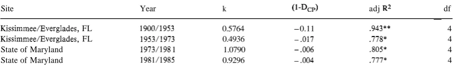
Table 2. Fractal cross-predictability dimension (stated as 1-Dcp, scale constant (k), adjusted R2, and degrees of freedom (df) from regression of equation 3 for cross-predictability (Pa for both data sets. ** indicates significant at the 0.1 level, * indicates significant at the .05 level.
Site Year k (I-Dcp) adj R2 df
~
Kissimmee/Everglades, FL 1900/1953 0.5764 -0.11 .943** 4
Kissimmee/Everglades, FL 1953/1973 0.4936 - .017 .778* 4
State of Maryland 1973/198 1 1.0790 - .006 .805* 4
State of Maryland 1981/1985 0.9296 - .004 .777* 4
where:
P = the spatial predictability (Pa refers to auto- predictability, Pc refers to cross-predicta- bility)
r = the resolution measured as the number of cells/km2
k = a scaling factor
D, = the fractal predictability dimension (dimen- sionless)
by first transforming it into log-log form:
In (PI) =
In
(k)+
(1 -D,)ln (r) (3)and using standard linear regression analysis to solve for the parameters k and D,.
The results are summarized in Table 1
,
which in- dicates the high R2 for this relationship for both of the study sites.Cross-predictability experiments
We calculated P, for both of the study areas by comparing maps from different years. This is ana-
logous to a simple “null model” that predicts land use patterns for one time from patterns at some previous time or times. This “model” includes no information on the underlying processes of change, but we were interested in how changing the resolu- tion of the maps affected the predictability, and the “null model” of no change is an interesting point of reference. We fit equation 3 to the data and the results for the three sites are shown in Table 2.
55
A: Kissimmee Everglades Basin, Florida
-3
,
..
t0 Pa 1900
x Pa 1953 + Pa 1973
pC I 900/1953 A P, 19531973
-1.1
’
.-6 -5 -4 -3 -2 -1 0 1
In(reso1ution)
B: State of Maryland
0
- 1 0 Pa 1973
x Pa 1981
+ P a 1985
0 Pc 1973/1981 A P, 1981/1985 h - 2
.-
5
- 3.-
Q 0
- 4
.-
-.9 J .
.
Ic
-5 -4 -3 -2 -1 0 1 2
In(reso1ution)
Fig. 3. Natural log of resolution vs. natural log of predictability for A) the Kississmee/Everglades, Florida, and B) the state of Maryland land use data. Plot shows both auto-predictability (Pa) indicating internal pattern in the data for three different years, and cross-predictability (P,) indicating pattern matching between null models of prior land use maps and the particular map. The resolutions used (in cells/kmZ) were: Florida: 0.005, 0.021, 0.083, 0.333, 1.333; Maryland: 0.011, 0.043, 0.171, 0.686, 2.743.
times that for the Maryland data. Auto-predicta- bility varied from about 0.65 to 0.35 over the range of resolutions used for the Florida data, but only from about 0.55 to 0.45 for the Maryland data. The Kissimmee/Everglades data was also more predic- table at the highest resolutions than the Maryland data.
The cross-predictability results also differ markedly between the Florida and Maryland data. The slope of the regression line (1 - D,, was about
three times higher for the Florida data than the Maryland data. Recall that the “null models” we are comparing with “data” in this analysis were
Model Predictability
(different models have different slopes and points of intersection)
I
I
Lower Higher
(larger grain) (smaller grain)
Ln of Resolution
Fig. 4. Hypothetical relationship between resolution and predic-
tability of data and models. Data predictibility is the degree to which the uncertainty about the state of landscape pixels is reduced by knowledge of the state of adjacent pixels in the same map. Model predictability is the degree to which the uncertainty about the state of pixels is reduced by knowledge of the cor- responding state of pixels in output maps from various models of the system.
land use data from prior years. As we can see from the results, this null model is a very good predictor of land use at all resolutions if the land use did not change radically over the study interval (as was the case in Maryland). In the Florida case, we were using a longer time interval and land use had changed radically over this interval, so the null model was much less accurate at all resolutions.
In addition, this “null model” is of limited real usefulness since it embodies none of the underlying processes that caused the land use changes in the first place. In the more general case of dynamic landscape models, or models in general, we would not expect such high initial values of predictability, and would expect the predictability to fall more quickly with resolution. We are currently building dynamic landscape models to test this hypothesis which can be summarized in Fig. 4.
Discussion and conclusions
We can draw several conclusions from our analysis: 1. Pa and P, belong to a class of “fractal-like”
56
dimension” to be calculated that permits easy conversion of measurements of P taken at one resolution to other resolutions (for example, resolutions higher than those for which we have data). We suspect that there are many other spatial measures, which also exhibit this kind of self-similarity, that may be useful in developing a generalized theory of scaling.
2. Pa generally increases with increasing resolu- tion. This relationship represents the “benefit” in terms of information gained about the pattern as resolution is increased.
3. P, generally falls with increasing resolution. This relationship represents the “cost” of de- creased model predictability as resolution is in- creased.
Combining 2 and 3 leads to some hypotheses about determining an “optimal” resolution for specific studies. At very low resolution it is easier to build predictive models, but they have little useful detail. At high resolution much useful de- tail is retained, but models are less able to predict it. An optimal resolution for scientific analysis may occur where these trends intersect - where one is balancing the costs and benefits incurred with increasing resolution. These results are con- sistent with empirical data from a survey of over
85 models of freshwater wetlands (Costanza and Sklar 1985).
The “models” we have analyzed so far are very primitive “null models” that one would expect to be different in overall predictability (P,) and in their fractal predictability dimensions (D )
cp
than more sophisticated process-based spatial models (Costanza et al. 1990). We suspect that there is a different optimal resolution for each class of models, and possibly for each particular set of modeling objectives. We also suspect that Pc and its associated D,, will change with chang- ing technology and modeling skills. We are cur- rently pursuing research aimed at addressing these questions by applying process-based spa- tial models at several different resolutions. These results may be generalizable to all forms of resolutions (spatial, temporal, and number of components) and may shed some interesting light on “chaotic” behavior in systems. When
looking across resolutions, chaos may be the low level of model predictability that occurs as a natural consequence of high resolution. Lower- ing model resolution can increase model predic- tability by averaging out some of the chaotic be- havior at the expense of losing detail about the phenomenon. For example, Sugihara and May (1990) found chaotic dynamics for measles epi- demics at the level of individual cities, but more predictable periodic dynamics for whole nations. The idea is not to maximize the resolution of analysis in order to “discover” this “unpredict- able” chaotic behavior, nor is it to maximize pre- dictability by ignoring details. Rather, the aim is to choose the resolution that maximizes the effectiveness of the model in balancing the con- flicting trends of data and model predictability with changing resolution.
Acknowledgments
This research was supported in part by NSF Grants BSR-8814272 titled: Response of a major land mar- gin ecosystem to changes in terrestrial nutrient in- puts, internal nutrient cycling, production and ex- port; and BSR-8906269 titled: Landscape model- ing: the synthesis of ecological processes over large geographic regions and long time scales. We thank L. Graham for significant contributions to com- puter programming early in the development of these ideas, and S. Tennenbaum, F.H. Sklar, and L. Wainger and an anonymous reviewer for provid- ing useful comments on earlier drafts. ,
References
Colwell, R.K. 1974. Predictability, constancy, and contingency of periodic phenomena. Ecology 55: 1148-1153.
Costanza, R. 1975. The spatial distribution of land use sub- systems, incoming energy and energy use in South Florida from 1900 to 1973. Master’s Research Project. Department of Architecture, University of Florida, Gainesville, FL. 204 pp. Costanza, R. 1979. Embodied energy basis for economic: ecologic systems. Ph.D. Dissertation. University of Florida, Gainesville, FL. 254 pp.
57
Costanza, R. and Sklar, F.H. 1985. Articulation, accuracy, and effectiveness of mathematical models: a review of freshwater wetland applications. Ecological Modeling 27: 45-68. Costanza, R., Sklar, F.H. and White, M.L. 1990. Modeling
coastal landscape dynamics. BioScience 40: 91 - 107. Mandelbrot, B.B. 1977. Fractals. Form, chance and dimension.
W.H. Freeman and Co., San Francisco, C.A.
Mandelbrot, B.B. 1983. The Fractal Geometry of Nature. W.H. Freeman and Co., San Francisco, CA.
Milne, B.T. 1988. Measuring the fractal dimension of land- scapes. Applied Mathematics and Computation 27: 67-79. Olsen, L.F. and Schaffer, W.M. 1990. Chaos versus noisy peri-
odicity: alternative hypotheses for childhood epidemics. Science 249: 499-504.
Sugihara, G. and May, R.M. 1990. Nonlinear forecasting as a way of distinguishing chaos from measurement error in time series. Nature 344: 734-741.
Turner, M.G. 1987. Spatial simulation of landscape changes in Georgia: a comparison of 3 transition models. Landscape
Turner, M.G., Costanza, R. and Sklar, F.H. 1989. Methods to Compare Spatial Patterns for Landscape Modeling and Anal- ysis. Ecological Modelling 48: 1-18.