Consequences of Volume Fraction of Dust Particles on Fluid Flow past a Porous Triangular Geometry

(1)

CONSEQUENCES OF VOLUME FRACTION OF DUST PARTICLES

ON FLUID FLOW PAST A POROUS TRIANGULAR GEOMETRY

D S SWETHA1_{, K R MADHURA}2

Department of Mathematics, PES University, Bangalore, India, Contact: shwetha−[email protected]

Research Scholar : East West Institute of Technology, VTU, Karnataka, India. 2_{Post Graduate Department of Mathematics, The National College, Jayanagar, Bangalore,}

Trans - Disciplinary Research Centre, National Degree College, Basavanagudi and The Florida International University, USA, Contact: [email protected]

Abstract: The present study focuses on the im-pact of volume fraction of dust particles on fluid flow through porous triangular channel. Laplace transform,

Fourier transform and Crank-Nicolson methods are applied to the non-dimensional equations of unsteady,

laminar, viscous, incompressible flow of dusty fluid in presence of magnetic field under different pressure

gradients such as impulsive motion, transition motion and motion for a finite time. Fluid and dust velocity

profiles are obtained both analytically and numerically

which exhibits the effects of fluid flow for the various pertinent parameters like Reynolds number, Hartmann

number, permeability of porous medium and volume fraction of dust particles. Detailed discussions has

been carried out for the consequences of physical pa-rameters on fluid flow and presented through tables and

graphs. For the numerical computation, the efficient mathematical tool Mathlab is used. Consideration of

triangular geometry has been justified by specifying its advantages over other geometries. Finally, skin

fric-tion at the boundaries are calculated.

Keywords: Dusty fluid, triangular chan-nel, volume fraction of dust particles, porous medium.

AMS Subject Classification (2000): 76T10, 76T15.

1. Introduction

The phenomenon of multi-phase flows are of great interest to the fluid dynamics community and has been extensively studied due to its tremendous applications

in water flooding, terahertz tomography, nuclear en-gineering, polymer fluids and slurries etc. In contrast to this and due to wide applications like squeezing a wet sponge, filtering water etc, porous medium has become an area of attention for scientists, engineers and mathematicians as well.

A substantial number of investigations have been con-ducted to understand the concept of volume fraction not only due to its industrial applications but also the errors which occurs in the motion of the fluids when it is not considered. As a consequence, Rudinger [1] has shown the inaccuracy introduced in a flow analysis of gas particles mixtures by ignoring the volume frac-tion of dust particles. Saffman [2] has contemplated the laminar flow of a dusty fluid by disregarding the volume fraction of the dust particles. Later, for a similar stream, Gupta and Gupta [3] have established the outcomes by taking the volume fraction of dust particles into consideration and gave the significance of volume fraction of dust particles on motion of fluids. Including to these investigations, authors like Kamel A Elshorbagy et al. [4] have investigated the effect of volume fraction on the liquid-liquid hydrocyclone performance. A hydrocyclone is a gadget to charac-terize, discrete or sort particles in a liquid suspension based on the ratio of their centripetal force to fluid re-sistance. Hydrocyclone discover its application in the partition of liquids of various densities. The mixture is injected into the hydrocyclone so as to make the vortex and relying on the relative densities of the two

(2)

Nomenclature:

−

→_u _{- velocity of the fluid phase} −→_v _{- velocity of the dust phase}

k- 6πa1µ- stokes resistance coefficient t- time

a1 -spherical radius of the dust particle m- mass of the dust particle N0 - number density of the dust particles δ- spin gradient viscosity φ- volume fraction of the dust particles ρ- density of the fluid

σ- electrical conductivity µ- the coefficient of viscosity of fluid particles

p- pressure of the fluid β0 - intensity of the imposed transverse magnetic field η - permeability of the porous medium ν - kinematic viscosity

Ha- Hartmann number Re- Reynolds number

U - characteristic velocity

stages, the centrifugal acceleration will cause the dis-persed phase to move far from or towards the central core of the vortex. The flow conduct in hydro-cyclone is very intricate. The complexity of fluid flow in the hydrocyclone is due to the fact that flow in a hydro-cyclone is a swirling turbulent multiphase flow.

V.Ramana Reddy Janke [8] et al. have presented a study on momentum and heat transfer behaviour of MHD flow of a nanofluid embedded with dust par-ticles past a cone and shows that enhancement in the volume fraction of dust particles reduces the mo-mentum boundary layer thickness. Rakesh kumar [10] has adopted perturbation method to derive exact solutions for the fluid and particle velocites for a two-dimensional laminar flow of an electrically conducting, viscous, incompressible fluid through a long channel under the influence of pulsatile pressure gradient tak-ing volume fraction of dust particles into account. To study dusty-visco elastic fluid flow, Saffman model and Oldyord model have been used by Debasish Dey [11] in a horizontal channel with volume fraction and energy dissipation. MHD impact on convective flow of dusty viscous fluid with volume fraction of dust par-ticles was examined by Ibrahim Saidu et al. [12] and they have predicted that velocity of liquid and dust particles decelerates with the increment in the perme-able parameter. R.K.Gupta and S.N.Gupta [13] have made an exhaustive theoritical study on unsteady flow of a dusty fluid through ducts and exhibits the promi-nence of volume fraction assortment for the validity of Saffman model.

The flow problems over various channel received much attention in recent years because of its various appli-cations in nature, engineering devices, industrial and chemical engineering such as rock crystals in molten lava, particles in emulsion paints, reinforcing parti-cles in polymers melts etc. A detailed comparision of numerical and analytical solutions are interpreted through performance analysis graphs by D.S.Swetha [14] et al. to study the impact of Beltrami effect on dusty fluid flow through hexagonal channel in pres-ence of porous medium. Anil Tripathi et al. [15] have explored the effect of magnetic field on the flow of dusty visco-elastic second order oldroyd fluid through a long rectangular channel by captivating very small Reynolds number. R.K.Khare [6] et al. have ob-served the variation of velocity of fluid and dust phases with magnetic field which may be used to control the movement of dusty particles in MHD flow of a non-newtonian fluid through an isoceles triangular channel. Using the same triangular geometry, flux and skin friction drag on the walls of the cylinder have been calucated for different pressure gradients by E. Rukmangadachari and P.V.Arunachalam [7]. The intrinsic decomposition of flow equations in Frenet frame field system are carried out by B.J.Gireesha [9] et al. and their conclusions were based on veloc-ity profiles for disperate values of time and number density. K.R.Madhura [5] et al. have employed vari-able separvari-able and Laplace transform techniques for solving governing non-dimensional partial differential equations to study the effects of porosity parameter involved with the aid of graphs.

(3)

The advantages of triangular channel are:

• An unstructured grid is a tessellation of a part of the Euclidian space by simple shapes such as triangles or tetrahedron in a irregular pattern. Grids of this type may be used in finite ele-ment analysis when the input to be analyzed has an irregular shape.

• The grid quality is a complex characteristic that determines the overall accuracy of solu-tion at a given number of grid points and at a given discretization scheme. The best ac-curacy is provided for the second order finite volume schemes if the unstructured grid is or-thogonal.

• The benifits of triangular cell is that one can produce an orthogonal grid to such an extent that cell shape does not deviate too far from equilateral and that sizes of any two neigh-bouring cells do not vary excessively.

The advantages of triangular channel over rectangular channel are:

A notch is a device used for measuring the rate of flow of a liquid through a small channel or tank. It is open-ing in the side of a measuropen-ing tank or reservoir extend-ing above the free surfaces.

• The expression for discharge for a right angled triangular notch is very simple.

• For low discharges, a triangular notch gives more accurate results than rectangular notch. • Reasonably stable value of discharge coeefi-cient over a wide range of operating conditions. • Ventilation of triangular notch is not required.

Motivated by above mentioned investigations and its applications in various fields of science and technol-ogy, it is of interest to discuss and analyze the effects of pertinent parameters on velocity fields. Hence, the study reported herein considers the impact of volume fraction on unsteady dusty fluid flow through traingu-lar channel in presence of porous medium. The flow phenomenon has been characterized with the help of flow parameters viz. volume fraction of dust particles, Hartmann number, Reynolds number, porous param-eter and the effects of these paramparam-eters on the veloc-ity fields have observed and the results are presented graphically and discussed quantitatively with the help of graphs and tables.

2. Mathematical Analysis

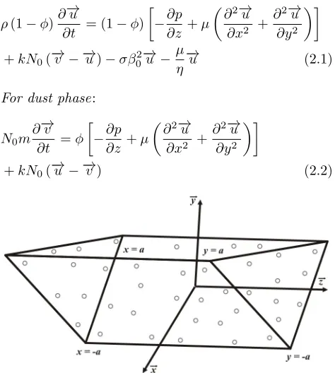
Consider an unsteady, laminar flow of a incompress-ible, viscous fluid through porous medium of a trian-gular channel with volume fraction of the dust particles taken into account and the governing equations of mo-tion are written in the following form :

For fluid phase:

ρ(1−φ)∂ − →_u

∂t = (1−φ)

−∂p

∂z +µ

_∂2−→_u ∂x2 +

∂2−→_u ∂y2

+kN0(−→v − −→u)−σβ02−→u − µ η

−

→_u _(2.1)

For dust phase:

N0m ∂−→v

∂t =φ

−∂p

∂z+µ

_∂2−→_u

∂x2 + ∂2−→_u

∂y2

+kN0(−→u − −→v) (2.2)

Fig. 1 : Schematic diagram of the dusty fluid flow through porous triangular channel

The following assumptions are made to analyze the flow :

• The volume fraction of dust particles (i.e. the volume occupied by the particles per unit vol-ume of the mixture) have been taken into con-sideration.

• The dust particles are spherical in shape, equal in size and uniformly distributed in the flow re-gion.

• Both the fluid and the dust particle clouds are static at the beginning.

• Using a triangular cartesian coordinate system (x, y, z) such thatz - axis is along the axis of the channel and the channel walls are bounded betweenx=−a, x=a, y=−a, y=a.

Taken into consideration of these assumptions for the flow through porous triangular channel, the velocity

(4)

distributions of fluid and dust particles are defined as:

→

u=uz

→

z , →v=vz

→

z (2.3)

i.e., ux =uy = 0 andvx=vy = 0 where (ux, uy, uz)

and (vx, vy, vz) denote the velocity components of

fluid and dust phases respectively.

Equations(2.1) and (2.2) are to be solved by subjecting to the initial and boundary conditions;

Initial condition : at t = 0, uz=vz= 0

Boundary condition: for t > 0,

uz =vz=g(t) at x=±a

uz =vz= 0 at y=±a (2.4)

The following are the dimensionless quantities and are defined as,

x=ax∗, y=ay∗,z=az∗, pa2₌_ρU2_p∗_,_tU ₌_a2_t∗_,

auz=U u∗z, avz=U vz∗;

Applying the above non-dimensional quantities, (2.1), (2.2) and boundary conditions becomes as follows;

∂uz

∂t =− ∂p ∂z+

a Re

_∂2_u

z

∂x2 + ∂2_u

z

∂y2

+1(vz−uz)

−Ha2ν U uz−

νa2

ηU(1−φ)uz (2.5)

∂vz

∂t =φ

0

−∂p

∂z + a Re

_∂2_u

z

∂x2 + ∂2uz

∂y2

+δ(uz−vz)

(2.6)

uz=vz=

a

U g(t) at x=±1

uz=vz= 0 at y=±1 (2.7)

where

Ha2 = σβ02a2

µ , f =

mN0

ρ , φ

0

= φ_f, δ = _mUka2,

=₍₁₋δ_φ₎, 1=f .

Let−∂p_∂z =℘(t) be the time dependent pressure gradi-ent to be imposed on the system.

By introducing Laplace transform technique to the above equations, following form exists :

s u=P(s) + a

Re

_∂2_u ∂x2+

∂2_u ∂y2

+1(v−u)

−Ha

2_ν

U u− νa2

ηU(1−φ)u (2.8)

s v=φ0 P(s) + a

Re ∂ u ∂x2+

∂ u

∂y2 +δ(u−v)

(2.9)

whereu=R∞

0 e

−st_u

zdt,v=R

∞

0 e

−st_v

zdt

Correspondingly boundary conditions emerges as :

u=v= a

U G(s) at x=±1

u=v= 0 at y=±1 (2.10)

where P(s) and G(s) is the laplace transform of ℘(t) andg(t) respectively.

Rearranging of equations (2.8) and (2.9) leads to :

s+Ha

2_ν

U +1+ νa2 ηU(1−φ)

u= a

Re

_∂2_u

∂x2+ ∂2_u ∂y2

+1v+P(s) (2.11)

_s₊_δ

φ0

v=P(s) + a

Re

_∂2_u ∂x2+

∂2_u ∂y2

+ δ

φ0u

(2.12)

Applying finite Fourier sine transform to equations (2.11), (2.12) and then to boundary conditions (2.10), equations reduces to following form :

∂2uF

∂x2 − Re

a

s+Ha

2_ν

U +1+ νa2 ηU(1−φ)+

ar2π2 Re

uF

+Re

a PF(s) + Re

a 1vF = 0 (2.13)

∂2_u

F

∂x2 + Re

a

_δ

φ0 − ar2_π2

Re

uF+

Re

a PF(s)− Re

a

_s₊_δ

φ0

vF = 0 (2.14)

uF =vF =

a

U GF(s) at x=±1

uF =vF = 0 at y=±1 (2.15)

where PF(s) and GF(s) are the finite Fourier sine

transform ofP(s) andG(s) and

uF =

Z 1

0

usin (rπx)dx, vF =

Z 1

0

vsin (rπx)dx

Letc1= Re_a

s+Ha_U2ν +1+ νa

2

ηU(1−φ)+

ar2_π2

Re

,

c2=Re_a 1, P

0

F(s) =

Re

a PF(s),c3=

Re a

δ

φ0 −

ar2π2 Re

,

c4=Re_a

s+δ φ0

(5)

Then the equations (2.13) and (2.14) can be written as:

∂2_u

F

∂x2 −c1uF+P

0

F(s) +c2vF = 0 (2.16)

∂2_u

F

∂x2 +c3uF +P

0

F(s)−c4vF = 0 (2.17)

Case-1 : Impulsive motion

In this case, considerg(t) =u0δ(t) and℘(t) =p0δ(t)

whereu0,p0are constants andδ(t) is Dirac-delta

func-tion. Then solutions obtained for (2.16) and (2.17) are

uF =

∞

X

r=1

au0(1−(−1)

r

) cosh(Ax)

rπUcosh (A) +

p0(1−(−1)

r

)

rπA2_a

×Re

1−cosh(Ax) cosh(A)

(2.18)

vF =

∞

X

r=1

au0(1−(−1)r) cosh(Ax)

rπUcosh (A) +

p0(1−(−1)r) rπA2_a

×Re

(2.19)

Inverse finite Fourier sine transform of equations (2.18) and (2.19) are

u= ∞ X r=1 2 _au

0(1−(−1)

r

) cosh(Ax)

rπUcosh (A) +

p0(1−(−1)

r

)

rπA2_a

×Re

sin(rπy) (2.20)

v= ∞ X r=1 2

au0(1−(−1)

r

) cosh(Ax)

rπUcosh (A) +

p0(1−(−1)

r

)

rπA2_a

×Re

sin(rπy) (2.21)

Applying inverse Laplace transform to equationsuand

v givesuz andvz as

uz=

∞ X r=1 ∞ X n=0

2a2_u

0(2n+ 1) (−1)

n

(1−(−1)r)

U r

×

cos(2n+1)₂ πx(C1+D1) sin (rπy)

Re + ∞ X r=1 ∞ X n=0

8p0 π2_r

×

(−1)n(1−(−1)r)cos(2n+1)₂ πx(C1+D1)

(2n+ 1)

×sin (rπy) (2.22)

vz=

∞ X r=1 ∞ X n=0

2a2_u

0(2n+ 1) (−1)n(1−(−1)r) U r

×

cos(2n+1)₂ πx(C2+D2) sin (rπy)

Re c2

+ ∞ X r=1 ∞ X n=0

8p0 π2_r

×

(−1)n(1−(−1)r)cos(2n+1)₂ πx(C2+D2)

(2n+ 1)c2

×sin (rπy) (2.23)

Shear stress (Skin friction): The explicit expres-sion for shear stress on the wall at x = ±1,y = ±1 respectively are given by:

D1,y=−

∞ X r=1 ∞ X n=0

a2_u

0πµ(2n+ 1)2(1−(−1)r) U r

×sin (rπy) (C1+D1)

Re − ∞ X r=1 ∞ X n=0

4p0µ(1−(−1)

r

)

πr

×(C1+D1) sin (rπy) (2.24)

D−1,y=

∞ X r=1 ∞ X n=0

a2_u

0πµ(2n+ 1)2(1−(−1)r) U r

×(C1+D1) sin (rπy)

Re + ∞ X r=1 ∞ X n=0

4p0µ(1−(−1)

r

)

πr

×(C1+D1) sin (rπy) (2.25)

Dx,±1=−

∞ X r=1 ∞ X n=0

2a2_u

0πµ(2n+ 1) (−1)

n+r

(1−(−1)r)

U

×

cos(2n+1)₂ πx(C1+D1)

Re − ∞ X r=1 ∞ X n=0

8p0µ(−1)

n+r

(2n+ 1)

×

(1−(−1)r)cos(2n+1)₂ πx(C1+D1)

π (2.26)

Case-2 : Transition motion

Consider g(t) =u0H(t)e−ωt and ℘(t) =p0H(t)e−ωt

whereu0,p0,ωare constants andH(t) is a Heaviside’s

unit step function. The results exists as :

uz=

∞

X

r=1

2au0e−ωt(1−(−1)

r

) cosh (K1x) sin (rπy) U rπcosh (K1)

+ ∞ X r=1 ∞ X n=0

2a2u0(2n+ 1) (1−(−1)

r

)cos(2n+1)₂ πx

U r

×(−1)

n

(C3+D3) sin (rπy)

Re +

∞

X

r=1

2Rep0e−ωtsin (rπy) K2

1arπ

(6)

×(1−(−1)

r

) (cosh (K1)−cosh (K1x))

cosh (K1)

+ ∞ X r=1 ∞ X n=0

8p0

×

(−1)n(1−(−1)r)cos(2n+1)₂ πx(C3+D3) sin (rπy)

(2n+ 1)π2_r

(2.28)

vz=

∞

X

r=1

2au0e−ωt(1−(−1)

r

) cosh (K1x) sin (rπy) c2U rπ

×

Re a

−ω+Ha_U2ν+1+ νa

2

ηU(1−φ)+

ar2_π2

Re

−K₁2

cosh (K1)

+ ∞ X r=1 ∞ X n=0

2a2u0(2n+ 1) (−1)

n

(1−(−1)r) (C4+D4) c2U r

×

cos(2n+1)₂ πxsin (rπy)

Re +

∞

X

r=1

2Rep0e−ωt(1−(−1)

r

)

c2

× h

cosh (K1)

−K2

1+Rea

−ω+Ha2ν

U +1+

νa2 ηU(1−φ)

cosh (K1)

+ar_Re2π2+ cosh (K1x)

K2 1− Re a

−ω+Ha_U2ν +1

K2 1

+_ηUνa₍₁₋2_φ₎+ar_Re2π2isin (rπy)

arπ + ∞ X r=1 ∞ X n=0

8p0(−1)

n

(2n+ 1)π2

×

(1−(−1)r)cos(2n+1)₂ πx(C4+D4) sin (rπy)

rc2

(2.29)

Shear stress (Skin friction): For this case, the expression for shear stress at x = ±1,y = ±1 respectively are given by:

D1,y=

∞

X

r=1

2au0µe−ωt(1−(−1)

r

)K1tanh (K1) sin (rπy) U rπ − ∞ X r=1 ∞ X n=0

a2_u

0µ(2n+ 1)2π(1−(−1)r) (C3+D3) U

×sin (rπy)

rRe −

∞

X

r=1

2Rep0µe−ωt(1−(−1)

r

) tanh (K1) K1a

×sin (rπy)

rπ − ∞ X r=1 ∞ X n=0

4p0µ(C3+D3) sin (rπy) r

×(1−(−1)

r ) π − ∞ X r=1

2au0µe−ωt(1−(−1)

r

) cos (rπy)

U

(2.30)

D−1,y=−

∞

X

r=1

2au0µe−ωt(1−(−1)

r

)K1tanh (K1) U r

×sin (rπy)

π +a 2_u 0πµ ∞ X r=1 ∞ X n=0

(2n+ 1)2(1−(−1)r)

U r

Re + 2Rep0µe

−ωt

∞

X

r=1

(1−(−1)r)

rπ

×tanh (K1) sin (rπy)

K1a

+ ∞ X r=1 ∞ X n=0

4p0µ(1−(−1)r) r

π −2au0µe

−ωt

∞

X

r=1

(1−(−1)r)

U

×cos (rπy) (2.31)

Dx,±1=−

∞

X

r=1

2au0µe−ωt(−1)r(1−(−1)r) cosh (K1x) Ucosh (K1)

+

∞

X

r=1

µ(−1)r(1−(−1)r) (cosh (K1)−cosh (K1x)) K2

1acosh (K1)

×2Rep0e−ωt+

∞ X r=1 ∞ X n=0

8p0µ(−1)n+r(1−(−1)r)

(2n+ 1)

×

cos(2n₂+1)x(C3+D3)

π −2a

2_u 0πµ ∞ X r=1 ∞ X n=0

(2n+ 1)

U

×

(−1)n+r(1−(−1)r)cos(2n+1)₂ πx(C3+D3)

Re

(2.32)

Case-3 : Motion for a finite time

Take g(t) = u0[H(t)−H(t−T)], ℘(t) = p0[H(t)−H(t−T)] whereu0,p0,ωare constants and H(t) is a heaviside’s unit step function. The solutions take the form

uz=

∞ X r=1 ∞ X n=0

2a2_u

0(1−(−1)

r

)cos(2n+1)₂ πx

U

×(2n+ 1) (−1)

n

(C5+D5) sin (rπy) rRe + 8p0

∞ X r=1 ∞ X n=0

(−1)n

(2n+ 1)π2_r

(2.33)

vz=

∞ X r=1 ∞ X n=0

2a2_u

0(1−(−1)

r

)cos(2n+1)₂ πx

U c2

×(2n+ 1) (−1)

n

(C6+D6) sin (rπy) rRe + 8p0

∞ X r=1 ∞ X n=0

(−1)n

×

(2n+ 1)π2_rc 2

(7)

Shear stress (Skin friction): For this case, the ex-pression for shear stress on the wall atx=±1,y=±1 reduces to:

D1,y=−

∞ X r=1 ∞ X n=0

a2u0πµ(2n+ 1) 2

(1−(−1)r) (C5+D5) U rRe

×sin (rπy)−

∞ X r=1 ∞ X n=0

4p0µ(1−(−1)

r

) (C5+D5) sin (rπy) πr

(2.35)

D−1,y=

∞ X r=1 ∞ X n=0

a2_u

0πµ(2n+ 1)2(1−(−1)r) (C5+D5) U rRe

×sin (rπy) +

∞ X r=1 ∞ X n=0

4p0µ(1−(−1)

r

) (C5+D5) sin (rπy) π

(2.36)

Dx,±1=−

∞ X r=1 ∞ X n=0

2a2u0πµ(2n+ 1) (−1)

n+r

(1−(−1)r)

U Re

×cos

₍₂_n_{+ 1)}_π

2 x

(C5+D5)−8p0µ

∞ X r=1 ∞ X n=0

(−1)n+r (2n+ 1)

(1−(−1)r)cos(2n+1)₂ πx(C5+D5)

πr (2.37)

3. Numerical Solutions

The system of coupled partial differential equations (2.5) and (2.6) subject to the boundary conditions (2.7) have been solved numerically using Crank Nicol-son technique. The essence of this method reduces the difficulties of time consumption and solving techniques. Therefore, here the mathematical software Mathlab has been used to obtain numerical solutions for the same prescribed flow. The governing equations are given by :

1 4t+

a

Re(4x)2 +

a

Re(4y)2 !

un_i,j+1− a 2Re(4x)2

u_in₊₁+1_,j+u_in₋+1₁_,j− a

2Re(4y)2 u

n+1

i,j+1+u

n+1

i,j−1

=℘(t) + 1 4t−

a

Re(4x)2−

a

Re(4y)2 −S1 !

un_i,j

+ a

2Re(4x)2 u

n

i+1,j+u

n i−1,j

+ a

2Re(4y)2 u

n i,j+1

+un_i,j₋₁

+1vi,jn (3.1)

1 4tv

n+1

i,j −

aφ0

2Re(4x)2 u

n+1

i+1,j+u

n+1

i−1,j

− aφ

0

2Re(4y)2

un_i,j+1₊₁+un_i,j+1₋₁

+ aφ

0

Re(4x)2 +

aφ0

Re(4y)2 !

un_i,j+1

=φ0℘(t) + − aφ

0

Re(4x)2 −

aφ0

Re(4y)2 +δ !

un_i,j

+ ₁

4t −δ

vni,j+

aφ0

2Re(4x)2 u

n

i+1,j+u

n i−1,j

+ aφ

0

2Re(4y)2 u

n

i,j+1 +u

n i,j−1

(3.2)

Case-1:

The corresponding initial and boundary conditions are given by :

For t= 0, u0_i,j=v0_i,j= 0

For t > 0, un₀_,j =v₀n_,j = a

Ug(t) at x=−1

un_n₁_,j =vn_n₁_,j = a

Ug(t) at x= 1 un_i,₀=vn_i,₀= 0 at y=−1

un_i,n₁=vn_i,n₁= 0 at y= 1

For this case, g(t) =u0δ(t) and℘(t) =p0δ(t) where u0andp0 are constants,δ(t) is Dirac-delta function.

Case-2:

The initial and boundary conditions changes to :

For t= 0, u0_i,j=v0_i,j= 0

For t > 0, un₀_,j =v₀n_,j = a

Ug(t) at x=−1

unn1,j =v

n

n1,j =

a

un_i,n

1=v

n

i,n1= 0 at y= 1

Here g(t) = u0H(t)e−ωt and ℘(t) = p0H(t)e−ωt

whereu0,p0,ωare constants andH(t) is a Heaviside’s

unit step function.

Case-3:

The initial and boundary conditions are represented as follows :

For t= 0, u0_i,j=v0_i,j= 0

For t > 0, un₀_,j =v₀n_,j = a

Ug(t) at x=−1

un_n

1,j =v

n

n1,j =

a

un_i,n

1=v

n

(8)

Let us assume, g(t) = u0[H(t)−H(t−T)]e−ωt and ℘(t) = p0[H(t)−H(t−T)]e−ωt where u0,p0,ω are

constants andH(t) is a Heaviside’s unit step function.

Here, triangular computational domain is used with grid point distribution at unequal spacing such that i refers to x, j refers to y with step size of 4x= 0.25, 4y= 0.25 and n refers to time t with its mesh4t= 0.05 was selected. Throughout our analysis for numer-ical and analytnumer-ical results, we have employed 4x = 0.25, 4y = 0.25,a = 0.25,u0 = 0.2,p0 = 0.2,U =

0.1,κ = 0.3,N0 = 0.1,r = 1,n = 1,m = 0.2,ν =

0.2,ρ= 0.1,T = 4,ω= 0.2,t= 0.2 and to judge the accuracy of the convergence and stability of numerical techniques, the outcomes have computed with smaller values of 4x,4y i.e., 4x = 0.50, 0.25, 0.125 etc. and4y = 0.50, 0.25, 0.125 etc. The computations are iterated until to meet the convergence criteria at the streamwise position. The tables [1-24] reveals the analytical and numerical solutions of fluid and dust velocities for different values of volume fraction, Hart-mann number, Reynolds number, porosity and noticed that there is a close agreement with these approaches and thus ensures the accuracy of the methods used.

4. Results and discussions

The impact of volume fraction of dust particles on dusty fluid flow through triangular channel has been investigated in the presence of porous medium. The governing partial differential equations (2.5) and (2.6) are solved analytically using Laplace trans-form, Fourier transform and numerically using Crank-Nicolson methods. The influence of various pertinent parameters like volume fraction, Hartmann number,

Reynolds number and porous parameter on fluid and dust velocity profiles have been shown graphically [2-25] and exhibited the values through tables [1-24]. It is worth mentioning that the results obtained from both the methods are well in agreement. It is evident from the graphs that,

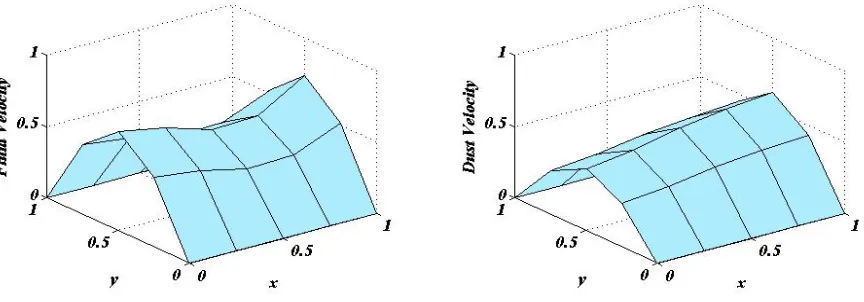
• The flow is parabolic in nature.

• The flow of fluid particles is parallel to that of dust.

• The fluid velocity is higher than the velocity of dust particles as dust particles restrict the flow.

The following results are obtained for the above three cases :

a. Impact of volume fraction on fluid and dust velocity profiles

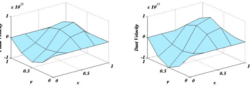
Figures [2-7] and tables [1-6] illustrates the effect of velocity profiles for different values of the volume frac-tion of dust particles. In order to maintain Saffman’s model, the range of volume fraction is choosen small. It is noticed from all the three cases that there is an impressive effect of volume fraction of dust particles on velocity fields i.e. the velocity profiles for both fluid and dust particles increases as volume fraction of dust particles increases. This phenomenon is observed as the volume occupied by the dust particles per unit volume of the fluid is higher than the dust concentra-tion i.e. fluid particles move faster than dust particles and also its effect is more prominent on the motion of dust particles, as the magnitude of the speed of dust particles increases but the dust particles experience a back flow.

y

Forφ= 0.04

Forx= 0.25 Forx= 0.50 Forx= 0.75

ua un va vn ua un va vn ua un va vn

0.25 -0.0183 -0.0184 -0.0153 -0.0153 0.0339 0.0340 0.0283 0.0284 0.0443 0.0445 0.0370 0.0371 0.50 -0.0259 -0.0260 -0.0217 -0.0219 0.0479 0.0479 0.0400 0.0401 0.0626 0.0628 0.0523 0.0525 0.75 -0.0183 -0.0184 -0.0153 -0.0153 0.0339 0.0340 0.0283 0.0284 0.0443 0.0445 0.0370 0.0371

(9)

y

Forφ= 0.06

Forx= 0.25 Forx= 0.50 Forx= 0.75

0.25 -0.0185 -0.0188 -0.0167 -0.0169 0.0342 0.0345 0.0308 0.0312 0.0447 0.0449 0.0403 0.0405 0.50 -0.0262 -0.0264 -0.0236 -0.0240 0.0484 0.0484 0.0436 0.0438 0.0632 0.0634 0.0570 0.0571 0.75 -0.0185 -0.0188 -0.0167 -0.0169 0.0342 0.0345 0.0308 0.0312 0.0447 0.0449 0.0403 0.0405

Table 2. Comparison of analytical and numerical solutions for fluid and dust velocity profiles for case-1

y

Forφ= 0.04

Forx= 0.25 Forx= 0.50 Forx= 0.75

0.25 0.4468 0.4469 0.3354 0.3355 0.3748 0.3749 0.3870 0.3871 0.3819 0.3820 0.4152 0.4155 0.50 0.6319 0.6320 0.4743 0.4744 0.5301 0.5302 0.5473 0.5474 0.5401 0.5402 0.5871 0.5872 0.75 0.4468 0.4469 0.3354 0.3355 0.3748 0.3749 0.3870 0.3871 0.3819 0.3820 0.4152 0.4155

y

Forφ= 0.06

Forx= 0.25 Forx= 0.50 Forx= 0.75

0.25 0.4587 0.4589 0.4089 0.4089 0.3834 0.3835 0.4719 0.4720 0.3876 0.3878 0.5036 0.5037 0.50 0.6488 0.6490 0.5782 0.5784 0.5422 0.5424 0.6674 0.6676 0.5482 0.5482 0.7122 0.7123 0.75 0.4587 0.4589 0.4089 0.4089 0.3834 0.3835 0.4719 0.4720 0.3876 0.3878 0.5036 0.5037

y

Forφ= 0.04

Forx= 0.25 Forx= 0.50 Forx= 0.75

0.25 -1.9005 -1.9006 -1.3076 -1.3078 3.5116 3.5118 2.4162 2.4165 4.5882 4.5883 3.1569 3.1570 0.50 -2.6877 -2.6880 -1.8492 -1.8495 4.9662 4.9665 3.4170 3.4172 6.4887 6.4888 4.4645 4.4647 0.75 -1.9005 -1.9006 -1.3076 -1.3078 3.5116 3.5118 2.4162 2.4165 4.5882 4.5883 3.1569 3.1570

y

Forφ= 0.06

Forx= 0.25 Forx= 0.50 Forx= 0.75

0.25 -1.9699 -1.9699 -2.6745 -2.6748 3.6399 3.6398 4.9418 4.9419 4.7557 4.7559 6.4567 6.4569 0.50 -2.7858 -2.7860 -3.7823 -3.7824 5.1475 5.1475 6.9887 6.9888 6.7256 6.7258 9.1312 9.1316 0.75 -1.9699 -1.9699 -2.6745 -2.6748 3.6399 3.6398 4.9418 4.9419 4.7557 4.7559 6.4567 6.4569

(10)

Fig. 2 : Variation of fluid and dust velocities whenφ= 0.04 for case-1

(11)

b. Impact of Hartmann number on fluid and dust velocity profiles

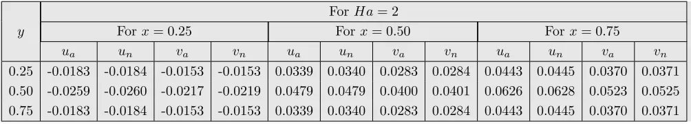
The influence of Hartmann number on velocity profiles are depicted in graphs [8-13] and tables [7-12] and re-veals that an increase in the Hartmann number results in depreciation of velocity phases of fluid and dust.

Physically, it is justified due to the fact that magnetic field normal to the flow direction prodcues a drag like or resistive force called Lorentz force which has a ten-dency to reduce fluid transport phenomena. This in turn generates lower velocity gradients in the channel. The same phenomenon is observed in all the cases.

(12)

y

ForHa= 2

Forx= 0.25 Forx= 0.50 Forx= 0.75

0.25 -0.0183 -0.0184 -0.0153 -0.0153 0.0339 0.0340 0.0283 0.0284 0.0443 0.0445 0.0370 0.0371 0.50 -0.0259 -0.0260 -0.0217 -0.0219 0.0479 0.0479 0.0400 0.0401 0.0626 0.0628 0.0523 0.0525 0.75 -0.0183 -0.0184 -0.0153 -0.0153 0.0339 0.0340 0.0283 0.0284 0.0443 0.0445 0.0370 0.0371

y

ForHa= 4

Forx= 0.25 Forx= 0.50 Forx= 0.75

0.25 -0.0004 -0.0003 -0.0083 -0.0081 0.0007 0.0008 0.0153 0.0154 0.0009 0.0009 0.0200 0.0201 0.50 -0.0005 -0.0006 -0.0117 -0.0118 0.0009 0.0009 0.0217 0.0218 0.0012 0.0014 0.0283 0.0285 0.25 -0.0004 -0.0003 -0.0083 -0.0081 0.0007 0.0008 0.0153 0.0154 0.0009 0.0009 0.0200 0.0201

y

ForHa= 2

Forx= 0.25 Forx= 0.50 Forx= 0.75

0.25 0.4468 0.4469 0.3354 0.3355 0.3748 0.3749 0.3870 0.3871 0.3819 0.3820 0.4152 0.4155 0.50 0.6319 0.6320 0.4743 0.4744 0.5301 0.5302 0.5473 0.5474 0.5401 0.5402 0.5871 0.5872 0.75 0.4468 0.4469 0.3354 0.3355 0.3748 0.3749 0.3870 0.3871 0.3819 0.3820 0.4152 0.4155

y

ForHa= 4

Forx= 0.25 Forx= 0.50 Forx= 0.75

0.25 0.1622 0.1623 0.3594 0.3595 0.1467 0.1469 0.3741 0.3745 0.1909 0.1908 0.3530 0.3532 0.50 0.2293 0.2295 0.5083 0.5084 0.2075 0.2078 0.5291 0.5292 0.2700 0.2702 0.4992 0.4994 0.75 0.1622 0.1623 0.3594 0.3595 0.1467 0.1469 0.3741 0.3745 0.1909 0.1908 0.3530 0.3532

y

ForHa= 2

Forx= 0.25 Forx= 0.50 Forx= 0.75

0.25 -1.9005 -1.9006 -1.3076 -1.3078 3.5116 3.5118 2.4162 2.4165 4.5882 4.5883 3.1569 3.1570 0.50 -2.6877 -2.6880 -1.8492 -1.8495 4.9662 4.9665 3.4170 3.4172 6.4887 6.4888 4.4645 4.4647 0.75 -1.9005 -1.9006 -1.3076 -1.3078 3.5116 3.5118 2.4162 2.4165 4.5882 4.5883 3.1569 3.1570

(13)

y

ForHa= 4

Forx= 0.25 Forx= 0.50 Forx= 0.75

0.25 -0.4406 -0.4409 -0.6091 -0.6095 0.8141 0.8142 1.1255 1.1256 1.0637 1.0638 1.4706 1.4709 0.50 -0.6231 -0.6235 -0.8615 -0.8615 1.1513 1.1514 1.5918 1.5919 1.5042 1.5044 2.0797 2.0798 0.75 -0.4406 -0.4409 -0.6091 -0.6095 0.8141 0.8142 1.1255 1.1256 1.0637 1.0638 1.4706 1.4709

Fig. 8 : Variation of fluid and dust velocities whenHa= 2 for case-1

(14)

c. Impact of Reynolds number on fluid and

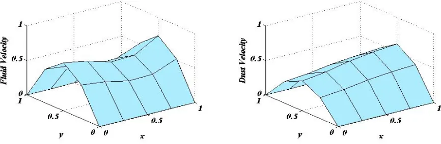
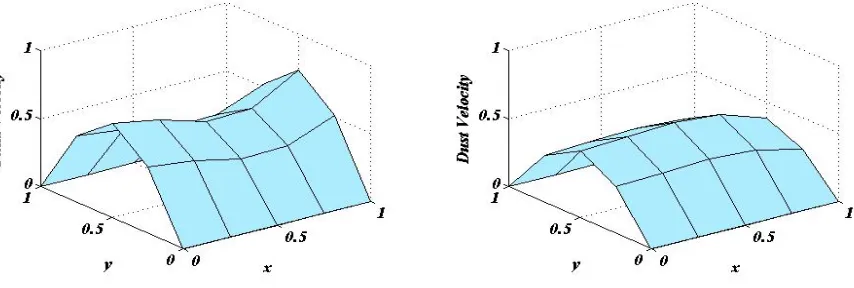
dust velocity profiles

The influence of the Reynolds number on fluid and dust velocity profiles have been demonstrated with the assist of graphs [14-19] and tables [13-18] and it is evi-dent from all the three cases that there is an apprecia-ble effect of Reynolds number on both velocity profiles

i.e., the velocity profiles for both fluid and dust par-ticles increases as Reynolds number increases. This behaviour is physically true, since Reynolds number is the measure of inertial force to viscous force. For the increasing values of Reynolds number, inertial forces are dominant over viscous forces and vice-versa, which inturn leads to increase of velocities of the flow.

(15)

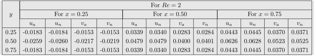
y

ForRe= 2

Forx= 0.25 Forx= 0.50 Forx= 0.75

0.25 -0.0183 -0.0184 -0.0153 -0.0153 0.0339 0.0340 0.0283 0.0284 0.0443 0.0445 0.0370 0.0371 0.50 -0.0259 -0.0260 -0.0217 -0.0219 0.0479 0.0479 0.0400 0.0401 0.0626 0.0628 0.0523 0.0525 0.75 -0.0183 -0.0184 -0.0153 -0.0153 0.0339 0.0340 0.0283 0.0284 0.0443 0.0445 0.0370 0.0371

y

ForRe= 4

Forx= 0.25 Forx= 0.50 Forx= 0.75

0.25 -0.0332 -0.0334 -0.0212 -0.0214 0.0614 0.0615 0.0392 0.0394 0.0803 0.0805 0.0513 0.0515 0.50 -0.0470 -0.0471 -0.0300 -0.0301 0.0869 0.0870 0.0555 0.0557 0.1135 0.1137 0.0725 0.0727 0.75 -0.0332 -0.0334 -0.0212 -0.0214 0.0614 0.0615 0.0392 0.0394 0.0803 0.0805 0.0513 0.0515

y

ForRe= 2

Forx= 0.25 Forx= 0.50 Forx= 0.75

0.25 0.4468 0.4469 0.3354 0.3355 0.3748 0.3749 0.3870 0.3871 0.3819 0.3820 0.4152 0.4155 0.50 0.6319 0.6320 0.4743 0.4744 0.5301 0.5302 0.5473 0.5474 0.5401 0.5402 0.5871 0.5872 0.75 0.4468 0.4469 0.3354 0.3355 0.3748 0.3749 0.3870 0.3871 0.3819 0.3820 0.4152 0.4155

y

ForRe= 4

Forx= 0.25 Forx= 0.50 Forx= 0.75

0.25 0.5967 0.5969 0.4369 0.4370 0.4628 0.4628 0.5055 0.5058 0.4305 0.4308 0.5144 0.5145 0.50 0.8439 0.8440 0.6178 0.6179 0.6545 0.6548 0.7149 0.7150 0.6088 0.6088 0.7275 0.7278 0.75 0.5967 0.5969 0.4369 0.4370 0.4628 0.4628 0.5055 0.5058 0.4305 0.4308 0.5144 0.5145

y

ForRe= 2

Forx= 0.25 Forx= 0.50 Forx= 0.75

0.25 -1.9005 -1.9006 -1.3076 -1.3078 3.5116 3.5118 2.4162 2.4165 4.5882 4.5883 3.1569 3.1570 0.50 -2.6877 -2.6880 -1.8492 -1.8495 4.9662 4.9665 3.4170 3.4172 6.4887 6.4888 4.4645 4.4647 0.75 -1.9005 -1.9006 -1.3076 -1.3078 3.5116 3.5118 2.4162 2.4165 4.5882 4.5883 3.1569 3.1570

(16)

y

ForRe= 4

Forx= 0.25 Forx= 0.50 Forx= 0.75

0.25 -1.0945 -1.0946 -1.6641 -1.6642 2.0223 2.0224 3.0749 3.0750 2.6423 2.6425 4.0176 4.0178 0.50 -1.5478 -1.5480 -2.3535 -2.3538 2.8600 2.8601 4.3486 4.3488 3.7368 3.7370 5.6817 5.6819 0.75 -1.0945 -1.0946 -1.6641 -1.6642 2.0223 2.0224 3.0749 3.0750 2.6423 2.6425 4.0176 4.0178

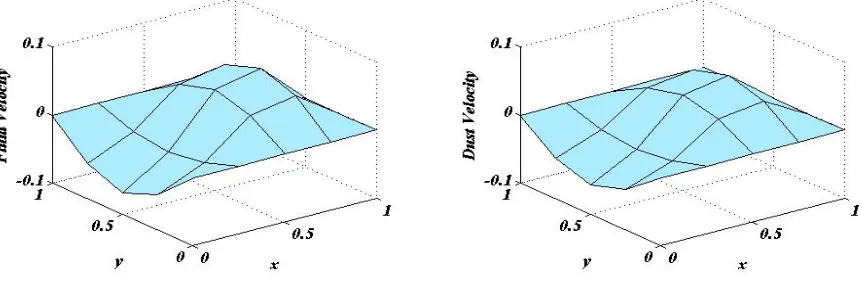
Fig. 14 : Variation of fluid and dust velocities when Re= 2 for case-1

(17)

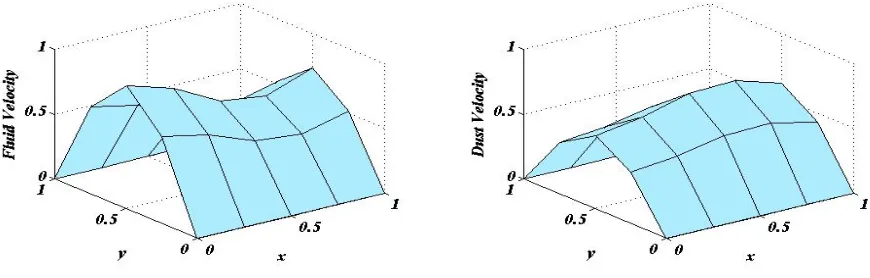
d. Impact of permeability of porous medium

on fluid and dust velocity profiles

Porosity is a crucial basic parameter for most charac-teristic and man made materials and fundementally impacts the physical properties of velocity, volume fraction and so forth. The porous parameter plays an vital role on velocity profiles of both fluid and dust particles. The increase in the porosity of the fluid and dust phases, seems have effect except in the case of mo-tion for a finite time where the velocities declines with

(18)

18 D S SWETHA, K R MADHURA

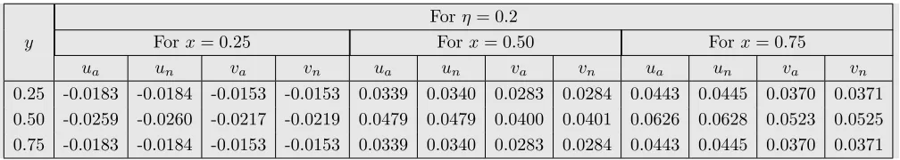
y

Forη= 0.2

Forx= 0.25 Forx= 0.50 Forx= 0.75

0.25 -0.0183 -0.0184 -0.0153 -0.0153 0.0339 0.0340 0.0283 0.0284 0.0443 0.0445 0.0370 0.0371 0.50 -0.0259 -0.0260 -0.0217 -0.0219 0.0479 0.0479 0.0400 0.0401 0.0626 0.0628 0.0523 0.0525 0.75 -0.0183 -0.0184 -0.0153 -0.0153 0.0339 0.0340 0.0283 0.0284 0.0443 0.0445 0.0370 0.0371

y

Forη= 0.4

Forx= 0.25 Forx= 0.50 Forx= 0.75

0.25 -0.0196 -0.0198 -0.0155 -0.0157 0.0361 0.0363 0.0287 0.0289 0.0472 0.0474 0.0375 0.0377 0.50 -0.0277 -0.0278 -0.0220 -0.0224 0.0511 0.0512 0.0406 0.0407 0.0668 0.0668 0.0530 0.0532 0.75 -0.0196 -0.0198 -0.0155 -0.0157 0.0361 0.0363 0.0287 0.0289 0.0472 0.0474 0.0375 0.0377

y

Forη= 0.2

Forx= 0.25 Forx= 0.50 Forx= 0.75

0.25 0.4468 0.4469 0.3354 0.3355 0.3748 0.3749 0.3870 0.3871 0.3819 0.3820 0.4152 0.4155 0.50 0.6319 0.6320 0.4743 0.4744 0.5301 0.5302 0.5473 0.5474 0.5401 0.5402 0.5871 0.5872 0.75 0.4468 0.4469 0.3354 0.3355 0.3748 0.3749 0.3870 0.3871 0.3819 0.3820 0.4152 0.4155

y

Forη= 0.4

Forx= 0.25 Forx= 0.50 Forx= 0.75

0.25 0.4571 0.4573 0.3365 0.3368 0.3828 0.3830 0.3864 0.3864 0.3875 0.3878 0.4122 0.4124 0.50 0.6464 0.6466 0.4758 0.4759 0.5414 0.5416 0.5464 0.5468 0.5480 0.5485 0.5830 0.5832 0.75 0.4571 0.4573 0.3365 0.3368 0.3828 0.3830 0.3864 0.3864 0.3875 0.3878 0.4122 0.4124

y

Forη= 0.2

Forx= 0.25 Forx= 0.50 Forx= 0.75

0.25 -1.9005 -1.9006 -1.3076 -1.3078 3.5116 3.5118 2.4162 2.4165 4.5882 4.5883 3.1569 3.1570 0.50 -2.6877 -2.6880 -1.8492 -1.8495 4.9662 4.9665 3.4170 3.4172 6.4887 6.4888 4.4645 4.4647 0.75 -1.9005 -1.9006 -1.3076 -1.3078 3.5116 3.5118 2.4162 2.4165 4.5882 4.5883 3.1569 3.1570

(19)

y

Forη= 0.4

Forx= 0.25 Forx= 0.50 Forx= 0.75

0.25 -0.5657 -0.5658 -0.4002 -0.4004 1.0454 1.0456 0.7394 0.7396 1.3658 1.3660 0.9661 0.9662 0.50 -0.8001 -0.8001 -0.5659 -0.5659 1.4784 1.4786 1.0457 1.0459 1.9316 1.9318 1.3662 1.3663 0.75 -0.5657 -0.5658 -0.4002 -0.4004 1.0454 1.0456 0.7394 0.7396 1.3658 1.3660 0.9661 0.9662

Fig. 20 : Variation of fluid and dust velocities whenη= 0.2 for case-1

(20)

5. Conclusions

The problem on dusty fluid flow through porous tri-angular channel has been studied. By using the ap-propriate transformation for the fluid and dust veloc-ities, the basic equations governing the flow were re-duced to set of partial differential equations. These

equations are solved analytically and numerically us-ing Laplace transform, Fourier transform and Crank-Nicolson methods. Some important conclusions ob-tained from this investigation are summarized as fol-lows:

(21)

• Graphs [2-25] and tables [1-24] elucidate the variation of the volume fraction of dust parti-cles, Hartmann number, Reynolds number and porosity on velocity profiles of fluid and dust for different boundary conditions as mentioned in case-1, case-2 and case-3.

• It is interesting to note that, the effect of volume fraction of dust particles on velocity phases of fluid and dust are same.

• The increasing in Hartmann number on ve-locity profiles results in decrease of veve-locity phases.

• There is an impressible effect of Reynolds num-ber on fluid and dust velocity profiles.

• The accelerating effect on fluid and dust veloc-ity profiles are observed in case-1 and case-2 whereas deaccelerating effect was there in the case of finite time as increasing the permeabil-ity of porous medium.

References

[1] Rudinger G,Some effects of finite particle volume on the dynamics of the gas-particle mixtures , AIAA J 3(7) (1962) 1217-1222.

[2] P.G. Saffman, On the stability of laminar flow of a dusty gas, Journal of fluid mechanics, Vol. 13(1), pp. 120-128, 1962.

[3] P.K.Gupta, S.C.Gupta,Flow of a dusty gas through a chan-nel with arbitrary time varying pressure gradient, J Appl Math Phys 27(1) (1976) 119-125.

[4] Kamel A Elshorbagy, Amr Abdelrazek and Mohamed Elsabaawy,Effect of volume fraction on the performance and separation efficiency of a de-oiling hydrocyclone, CFD Letters, Vol 5(4)-Dec 2013.

[5] K.R.Madhura, B.J.Gireesha, C.S.Bagewadi,Flow of an un-steady dusty fluid through porous media in a channel of tri-angular cross-section, International Review of Physics, Vol 4, N.6-Dec(2010).

[6] Sana Ahsan, R.K.Khare, Ajit Paul,MHD flow of an non-mewtonian fluid through an isoceles triangular chan-nel, International journal of Emerging Technology and In-novative Engineering, Vol 1(7), 2015.

[7] E.Rukmangadachari, P.V.Arunachalam,Dusty viscous flow through a cylinder of triangular cross-section, Proc. Indian Acad. Sci, Vol 88, pp-169-179, 1979.

[8] V Ramana Reddy Jankea, Sandeep Naramgarib, Sugu-namma Vangalaa,MHD flow of a nanofluid embedded with dust particles due to cone with volume fraction of dust and nano particles, International conference on Computational Heat and Mass Transfer-2015.

[9] Mahesha, B.J.Gireesha, G.K.Ramesh, C.S.Bagewadi,Unsteady flow of a dusty fluid through a channel having triangular cross section in Frenet frame field system, Acta Universities Apulensis, Vol 25, pp-53-75. [10] Rakesh Kumar,Particulate couette flow with volume frac-tion of dust particles, Journal of Chemical, Biological and Physical Sciences 5(3) (2015) 2851-2862.

[11] Debasish Dey,Dusty hydromagnetic Oldyord fluid flow in a horizontal channel with volume fraction and energy dissi-pation, International Journal of Heat and Technology, Vol 34(3), 415-422.

[12] I.Saidu, M.Y.Waziri, A.Roko, H.Musa, MHD effects on convective flow of dusty viscous fluid with volume frac-tion of dust particles, ARPN J. of Engg. and Applied Sci-ences, 5(10) (2010), 86-91.

[13] R.K.Gupta, S.N.Gupta,Unsteady flow of a dusty fluid through ducts with volume fraction, Proc. Indian natn. Sci. Acad, A 4 (1984) 350-364.

[14] K.R.Madhura, D.S.Swetha, S.S.Iyengar,The impact of Bel-trami effect on dusty fluid flow through hexagonal channel in presence of porous medium, Applied Mathematics and Computation, Vol 313, 342-354.

[15] Anil Tripathi, A.K.Sharma, K.K.Singh,Effect of porous medium and magnetic field on the flow of dusty visco-elastic second order oldroyd fluid through a long rectangular channel, International Journal of Mathematical Archive, 4(9) (2013), 243-247.

(22)

6. Appendix

c12=

δRe−φ0ar2π2, c13=

_Ha2_ν U +1+

νa2 ηU(1−φ)+

ar2π2 Re

y1=

−b11+

p

b2

11−4a11c11

2a11

, y2=

−b11−

p

b2

11−4a11c11

2a11

, K1=

s

Re(ω2₋_ω₍_c

13+δ) +c14) a(1φ

0

−ω+δ)

a11= 4Re, b11= 4Rec13+ 4Reδ+a(2n+ 1)2π2, c11= 4Rec14+a1φ

0

(2n+ 1)2π2+δa(2n+ 1)2π2

C1=

ey1t

1φ

0

+y1+δ

2

[(1φ

0

+y1+δ)(2y1+c13+δ)−(y21+y1(c13+δ) +c14)]

D1=

ey2t

1φ

0

+y2+δ

2

[(1φ0+y2+δ)(2y2+c13+δ)−(y22+y2(c13+δ) +c14)]

C2= ey1t

1φ

0

+y1+δ

2

Re a

y1+Ha

2_ν

U +1+ νa

2

ηU(1−φ)+

ar2_π2

Re

+(2n+1)₄ 2π2

[(1φ

0

+y1+δ)(2y1+c13+δ)−(y21+y1(c13+δ) +c14)]

D2= ey2t

1φ

0

+y2+δ

2

Re a

y2+Ha

2_ν

U +1+

νa2

ηU(1−φ)+

ar2_π2

Re

+(2n+1)₄ 2π2

[(1φ

0

+y2+δ)(2y2+c13+δ)−(y22+y2(c13+δ) +c14)]

C3=

ey1t

1φ

0

+y1+δ

2

(y1+ω) [(1φ

0

+y1+δ)(2y1+c13+δ)−(y12+y1(c13+δ) +c14)]

D3=

ey2t

1φ

0

+y2+δ

2

(y2+ω) [(1φ

0

+y2+δ)(2y2+c13+δ)−(y22+y2(c13+δ) +c14)]

C4= ey1t

1φ

0

+y1+δ

2

Re a

y1+Ha

2_ν

U +1+

νa2

ηU(1−φ)+

ar2π2 Re

+(2n+1)₄ 2π2

(y1+ω) [(1φ

0

+y1+δ)(2y1+c13+δ)−(y21+y1(c13+δ) +c14)]

D4= ey2t

1φ

0

+y2+δ

2

Re a

y2+Ha

2_ν

U +1+

νa2

ηU(1−φ)+

ar2π2 Re

+(2n+1)₄ 2π2

(y2+ω) [(1φ

0

+y2+δ)(2y2+c13+δ)−(y22+y2(c13+δ) +c14)]

C5=

ey1t

1φ

0

+y1+δ

2

(1−e−y1T₎

y1[(1φ

0

+y1+δ)(2y1+c13+δ)−(y12+y1(c13+δ) +c14)]

D5=

ey2t

1φ

0

+y2+δ

2

(1−e−y2T₎

y2[(1φ0+y2+δ)(2y2+c13+δ)−(y22+y2(c13+δ) +c14)]

C6= ey1t

1φ

0

+y1+δ

2

(1−e−y1T₎

Re a

y1+Ha

2_ν

U +1+ νa

2

ηU(1−φ)+

ar2_π2

Re

+(2n+1)₄ 2π2

y1[(1φ

0

+y1+δ)(2y1+c13+δ)−(y21+y1(c13+δ) +c14)]

D6= ey2t

1φ

0

+y2+δ

2

(1−e−y2T₎

Re a

y2+Ha

2_ν

U +1+

νa2

ηU(1−φ)+

ar2_π2

Re

+(2n+1)₄ 2π2

y2[(1φ

0

+y2+δ)(2y2+c13+δ)−(y22+y2(c13+δ) +c14)]

S1= Ha2_ν