Modelling of Biserial Bulk Queue Network Linked With Common Server

(1)

ISSN: 2231-5373

http://www.ijmttjournal.org

Page 430

Modelling of Biserial Bulk Queue Network

Linked With Common Server

Meenu Mittal#1, Renu Gupta*2

#

Assistant Professor of Mathematics

Maharishi Markandeshwar (Deemed to be University), Mullana (Ambala), India *Research Scholar in Mathematics

Maharishi Markandeshwar (Deemed to be University), Mullana (Ambala), India

Abstract— Queuing theory continues to be one of the most extensive theories of stochastic models. Advanced theoretical models are being developed through innovative analytical study with vast applications. The present paper deals with the modelling of biserial bulk queue network with fixed batch size and connected with a common server. Performance measure of the model has been analysed in stochastic environment. Numerical illustration is provided to understand the model in a better way.

Keywords — Batch arrival, queue characteristics, stochastic environment.

I. INTRODUCTION

The initial study of queuing theory was carried out by A.K. Erlang [1]. The multi input idea in queuing theory was introduced by Pandey [2]. Jackson [3] derived the differential difference equations and obtained the steady state equations. The transient solution of a queue network model consisting of two queues in series was studied by O’Brein [4] with poisson input and exponential holding time. Queuing problems with batch arrival was studied by Suzuki [5]. The basic concept of biserial queuing system into the theory of queues was introduced by Maggu ([6], [7]). Further the transient analysis of serial queues under service parameter constraints was discussed by Maggu [8]. Two biseries queues with batch arrival at each stage were studied by Hafiz Noor Mohammad et.al. [9].

Singh T.P. and Kumar Vinod et.al. [10] studied the transient behaviour of a queuing network with parallel biseries queues. Further Singh T.P. and Gupta Deepak [11] analysed a queue network model comprised of biserial and parallel channel linked with a common server. The queue network model having batch arrival with threshold effect was studied by Mittal Meenu et.al. [12]. Later on priority queue model along intermediate queue under fuzzy environment with application was studied by Mittal Meenu et.al.[13] and Singh T.P., Kusum & Gupta Deepak [14] studied the feedback queue model where service rate were assumed propotional to queue numbers .The present paper is further an extension of the study made by Hafiz Noor Mohammad et.al. [9] in the sense that this paper deals with modelling of biserial bulk queue network with fixed size batch arrival and connected with a common server. Performance measure of the model has been analysed in stochastic environment. To understand the model in a better way numerical illustration is provided.

II. Description of the model

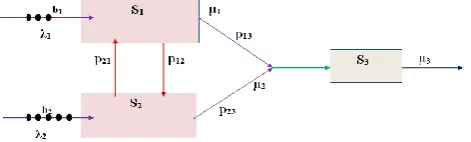
The queue network model in the problem consists of three service channels S1, S2, and S3.The S1 and S2

are biseries service channelswith queues q1 and q2 in front of these channels respectively. The third

service channel S3 is commonly linked with these two service channels.

Fig. 1

Biserialbulk queue network model linked with common server

The customers demanding service arrive in batches of fixed sizes b1 and b2 with arrival rates λ1 and λ2

under poisson assumption and joins the queues q1 and q2 respectively. The mean service rates at these

(2)

ISSN: 2231-5373

http://www.ijmttjournal.org

Page 431

Customers coming at rate λ1 after completion of service at S1 will either join S2 or S3 with the

probabilities p12 or p13 such that p12 + p13 = 1 and those coming at the rate λ2 after completion of service at

S2 will join either S1 or S3 with the probabilities p21 or p23 such that p21 + p23 =1 respectively. After

completion of service at S3 the customer is allowed to depart from the system.

A. Practical Situations

Many practical situations of model arise in banking system, administrative setup, club management, handling of children park, supermarket and production management etc. For example, suppose a game club consists of three sections S1, S2 & S3. The sections S1 and S2 provide the facility to play the games.

Both the games can be played only with a team of fixed size say b1 & b2 respectively. The customers

entering into the club either may join the section S1 or S2. Also there is a chance that a customer can either

move from one game to another or directly towards the section S3 for security measures.

B. Mathematical Analysis

The differential difference equations in transient form are as follows:

P´n₁.n₂.n₃ (t) = − (λ1+λ2+µ₁+µ2+µ3) Pn₁.n₂.n₃ (t) + λ1Pn₁-b₁.n₂.n₃ (t) + λ2Pn₁. n₂-b₂.n₃ (t)

+ µ1 p12 Pn₁+1.n₂-1.n₃ (t) + µ1p13 Pn₁+1. n₂. n₃ ₋1(t) + µ2 p21 Pn₁-1.n₂+1.n₃(t)

+ µ2 p23 Pn₁.n₂ +1.n₃ ₋1 (t) + µ3 Pn₁. n₂. n₃+1(t) (1)

for (n₁ > b₁ , n₂ > b2, n₃ > 0 )

P´n₁. n₂. n₃ (t) = − (λ1+λ2+µ₁+µ2+µ3) Pn₁.n₂.n₃ (t) + λ1 Pn₁-b₁.n₂.n₃ (t)+ µ1 p12 Pn₁+1.n₂-1.n₃(t) + µ1 p13 Pn₁+1.n₂.n₃ ₋1(t) + µ2 p21 Pn₁-1. n₂+1. n₃(t)+ µ2 p23 Pn₁.n₂ +1.n₃ ₋1(t)

+ µ3 Pn₁. n₂. n₃+1(t) (2)

for(n₁ > b₁ , n₂ < b2, n₃ > 0

)

P´n₁.0.n₃ (t) = − (λ1+λ2+µ₁ +µ3) Pn₁.0.n₃ (t) + λ1 Pn₁-b₁.0.n₃ (t) + µ1 p13 Pn₁+1.0.n₃ ₋1(t)

+ µ2 p21 Pn₁-1.1.n₃ (t) + µ2 p23 Pn₁.1.n₃ ₋1 (t) + µ3 Pn₁.0.n₃+1 (t) (3)

for(n₁ > b₁ , n₂ = 0, n₃ > 0)

P´n₁. n₂. 0(t) = − (λ1+λ2+µ₁ +µ2) Pn₁.n₂.0 (t) + λ1 Pn₁-b₁.n₂.0 (t) + λ2 Pn₁. n₂-b₂. 0 (t)

+ µ1 p12 Pn₁+1.n₂-1.0 (t)+ µ2 p21 Pn₁-1.n₂+1.0 (t) + µ3 Pn₁. n₂.1 (t) (4)

for(n₁ > b₁, n₂ > b2, n₃ = 0)

P´n₁. n₂.0(t) = − (λ1+λ2+µ₁ +µ2) Pn₁.n₂.0 (t) + λ1 Pn₁-b₁.n₂.0 (t) + µ1 p12 Pn₁+1. n₂-1.0 (t)

+ µ2 p21 Pn₁-1. n₂+1. 0 (t) + µ3 Pn₁.n₂.0 (t)

(5)

for(n₁ > b₁ , n₂ < b2, n₃ = 0)

P´n₁.0.0 (t) = − (λ1+λ2 +µ₁ ) Pn₁.0.0 (t) + λ1 Pn₁-b₁.0.0 (t) + µ2 p21 Pn₁-1.1.0 (t)

+µ3Pn₁.0.1(t) (6)

for(n₁ > b₁ , n₂ = 0, n₃ = 0)

P´0.n₂.n₃ (t) − (λ1+λ2+µ2+µ3) P0.n₂.n₃ (t) + λ2 P0. n₂-b₂. n₃ (t) + µ1 p12 P1. n₂-1. n₃ (t)

+µ1p13P1.n₂.n₃ ₋1(t) + µ2p23P0.n₂+1.n₃ ₋1(t)

+µ3P0.n₂.n₃+1(t) (7)

for(n₁ = 0, n₂ > b2, n₃ > 0)

P´0.n₂.n₃ (t) = − (λ1+λ2+µ2+µ3)P0.n₂.n₃ (t) + µ1 p12 P1. n₂-1. n₃ (t) + µ1 p13 P1. n₂. n₃ ₋1 (t)

+ µ2 p23 P 0. n₂ +1. n₃ ₋1 (t) + µ3 P0. n₂. n₃+1(t) (8)

for(n₁ = 0, n₂ < b2, n₃ > 0)

P´0.0.n₃ (t) = − (λ1+λ2+µ3) P0.0.n₃ (t) + µ1 p₁ ₃ P1. 0. n₃ ₋1(t) + µ2 p23 P0.1.n₃ ₋1(t)

+ µ3 P0. 0. n₃+1(t) (9)

for(n₁ = 0, n₂ = 0, n₃ > 0 )

P´0.n₂.0 (t) = − (λ1+λ2+µ2) P0.n₂.0 (t) + λ2 P0. n₂-b₂. 0 (t) + µ1 p12 P1. n₂-1. 0 (t)

+ µ3 P0.n₂.1(t) (10)

for(n₁ = 0, n₂ > b2, n₃ = 0)

P´0.n₂.0 (t) = − (λ1+λ2+µ2) P0.n₂.0 (t) + µ1 p12 P0. n₂-1. 0 (t)

+ µ3 P0. n₂. 1 (t) (11)

for(n₁ = 0, n₂ < b2, n₃ = 0)

(3)

ISSN: 2231-5373

http://www.ijmttjournal.org

Page 432

for(n₁ = 0, n₂ = 0, n₃ = 0)

P´n₁.n₂.n₃ (t) = − (λ1+λ2+µ₁ +µ2+µ3) Pn₁.n₂.n₃ (t) + λ2 Pn₁. n₂-b₂. n₃ (t) +

µ1 p12 Pn₁+1. n₂-1.n₃(t) + µ1 p13 Pn₁+1. n₂. n₃ ₋1(t) + µ2 p21 Pn₁-1. n₂+1. n₃ (t)

+µ2p23Pn₁.n₂+1.n₃ ₋1(t)+µ3Pn₁.n₂.n₃+1(t) (13)

for(n₁ < b₁, n₂ > b2, n₃ > 0)

P´n₁.n₂.n₃ (t) = − (λ1+λ2+µ₁+µ2+µ3) Pn₁.n₂.n₃ (t) + µ1 p12 Pn₁+1.n₂-1.n₃ (t)

+ µ1 p13 Pn₁+1.n₂.n₃ ₋1 (t) + µ2 p21 Pn₁-1.n₂+1.n₃ (t) + µ2 p23 Pn₁. n₂ +1.n₃ ₋1 (t)

+ µ3 Pn₁.n₂.n₃+1 (t) (14)

for(n₁ < b₁, n₂ < b2, n₃ > 0)

P´n₁.0.n₃ (t) = − (λ1+λ2+µ₁ +µ3)Pn₁.0.n₃ (t) + µ1 p13 Pn₁+1.0.n₃ ₋1 (t) + µ2 p21 Pn₁-1.1.n₃ (t)

+ µ2 p23 Pn₁.1.n₃ ₋1(t) + µ3Pn₁.0.n₃+1 (t) (15)

for(n₁ < b₁ , n₂ = 0, n₃ > 0)

P´n₁.n₂.0 (t) = − (λ1+λ2 +µ₁ +µ2)Pn₁.n₂.0 (t) + λ2 Pn₁. n₂-b₂. 0 (t) + µ1 p12 Pn₁+1.n₂-1.0 (t)

+ µ2 p21 Pn₁-1. n₂+1. 0 (t) + µ3 Pn₁. n₂.1 (t) (16)

for(n₁ < b₁ , n₂ > b2, n₃ = 0 )

P´n₁.n₂.0 (t) = − (λ1+λ2+µ₁+µ2)Pn₁.n₂.0 (t) + λ2 Pn₁.n₂-b₂.0 (t) + µ1 p12 Pn₁+1.n₂-1.0 (t)

+ µ2 p21 Pn₁-1.n₂+1.0 (t) + µ3 Pn₁.n₂.1 (t) (17)

for(n₁ < b₁ , n₂ < b2, n₃= 0)

P´n₁.0.0 (t) = − (λ1+λ2+µ₁)Pn₁.0.0 (t) + µ2 P21 Pn₁-1.1.0 (t) +µ3 Pn₁.n₂.1 (t) (18)

for(n₁ < b₁ , n₂ = 0, n₃= 0 )

Taking limit as 𝑡 →∞, corresponding steady state equations are as follows:

(λ1+λ2+µ₁ +µ2+µ3)Pn₁.n₂.n₃ = λ1 Pn₁-b₁. n₂. n₃ + λ2 Pn₁. n₂-b₂. n₃ + µ1 p12 Pn₁+1. n₂-1. n₃

+ µ1 p13 Pn₁+1. n₂. n₃ ₋1 + µ2 p21 Pn₁-1. n₂+1.n₃ + µ2 p23 Pn₁. n₂ +1. n₃ ₋1

+ µ3Pn₁. n₂. n₃+1 (19)

for(n₁ > b₁ , n₂ > b2, n₃ > 0 )

(λ1+λ2+µ₁ +µ2+µ3) Pn₁.n₂.n₃ = λ1 Pn₁-b₁. n₂. n₃ + µ1 p12 Pn₁+1. n₂-1. n₃+ µ1 p13 Pn₁+1. n₂. n₃ ₋1

+ µ2 p21 Pn₁-1.n₂+1.n₃+µ2 p23 Pn₁.n₂+1.n₃ ₋1+ µ3 Pn₁. n₂. n₃+1 (20)

for(n₁ > b₁ , n₂ < b2, n₃ > 0)

(λ1+λ2+µ₁ +µ3) Pn₁.0.n₃ = λ1 Pn₁-b₁.0.n₃ + µ1 p13 Pn₁+1. 0. n₃ ₋1 + µ2 p21 Pn₁-1. 1. n₃

+ µ2 p23 Pn₁.1.n₃ ₋1 + µ3Pn₁.0.n₃+1 (21)

for(n₁ > b₁ , n₂ =0, n₃ > 0)

(λ1+λ2+µ₁ +µ2) Pn₁.n₂.0 = λ1 Pn₁-b₁. n₂.0 + λ2 Pn₁. n₂-b₂. 0 + µ1 p12 Pn₁+1. n₂-1. 0

+ µ2 p21 Pn₁-1.n₂+1.0 + µ3 Pn₁. n₂.1 (22)

for(n₁ > b₁, n₂ > b2, n₃ = 0)

(λ1+λ2+µ₁ +µ2) Pn₁.n₂.0 = λ1 Pn₁-b₁. n₂. 0 + µ1 p12 Pn₁+1. n₂-1. 0 + µ2 p21 Pn₁-1. n₂+1. 0

+ µ3 Pn₁. n₂. 0 (23)

for(n₁ > b₁ , n₂ < b2, n₃ = 0)

(λ1+λ2+µ₁ ) Pn₁.0.0 = λ1 Pn₁-b₁.0.0 + µ2 p21 Pn₁-1.1.0 + µ3Pn₁.0.1 (24)

f

or(n₁ > b₁, n₂ = 0, n₃ = 0)

(λ1+λ2+µ2+µ3)P0.n₂.n₃ = λ2 P0. n₂-b₂. n₃ + µ1 p12 P1. n₂-1. n₃ + µ1 p13 P1. n₂. n₃ ₋1

+ µ2 p23 P0. n₂ +1. n₃ ₋1 + µ3 P0. n₂. n₃+1 (25)

for(n₁ = 0, n₂ > b2, n₃ > 0)

(λ1+λ2+µ2+µ3) P0.n₂.n₃ = µ1 p12 P1. n₂-1. n₃ + µ1 p13 P1. n₂. n₃ ₋1 + µ2 p23 P 0. n₂ +1. n₃ ₋1

+ µ3 P0. n₂. n₃+1 (26)

for(n₁ = 0, n₂ < b2, n₃ > 0)

(λ1+λ2+µ3)P0.0.n₃= µ1p13P1.0.n₃ ₋1+µ2p23P0.1.n₃ ₋1+µ3P0.0.n₃+1 (27)

for(n₁ = 0, n₂ = 0, n3 > 0 )

(λ1+λ2+µ2) P0.n₂.0 = λ2 P0.n₂-b₂.0 + µ1 p12 P1. n₂-1. 0 + µ3P0. n₂. 1 (28)

for(n₁ = 0, n₂ > b2, n3 = 0)

(λ1+λ2+µ2) P0.n₂.0 = µ1 p12 P0. n₂-1. 0 + µ3 P0. n₂. 1 (29)

for(n₁ = 0, n₂ < b2, n3 = 0)

(λ1+λ2) P0.0.0 = µ3 P0. 0. 1 (30)

for(n₁ = 0, n₂ = 0, n3 = 0)

(4)

ISSN: 2231-5373

http://www.ijmttjournal.org

Page 433

+ µ2 p21 Pn₁-1. n₂+1. n₃ + µ2 p23 Pn₁.n₂ +1.n₃ ₋1 + µ3 Pn₁. n₂. n₃+1 (31)

for(n₁ < b₁ , n₂ > b2, n3 > 0)

(λ1+λ2+µ₁ +µ2+µ3) Pn₁.n₂.n₃ = µ1 p12 Pn₁+1.n₂-1.n₃ + µ1 p13 Pn₁+1.n₂.n₃ ₋1

+µ2 p21 Pn₁-1. n₂+1. n₃ + µ2 p23 Pn₁. n₂ +1. n₃ ₋1 + µ3Pn₁. n₂. n₃+1 (32)

for(n₁ < b₁, n₂ < b2, n₃ > 0)

(λ1+λ2+µ₁ +µ3) Pn₁.0.n₃ = µ1p13 Pn₁+1.0.n₃ ₋1 + µ2 p21 Pn₁-1.1.n₃ + µ2 p23 Pn₁.1.n₃ ₋1

+ µ3Pn₁. 0. n₃+1 (33)

for(n₁ < b₁, n₂ = 0, n₃ > 0 )

(λ1+λ2+µ₁ +µ2) Pn₁.n₂.0 = λ2 Pn₁. n₂-b₂. 0 + µ1 p12 Pn₁+1. n₂-1. 0 + µ2 p21 Pn₁-1.n₂+1.0

+ µ3 Pn₁. n₂.1 (34)

for(n₁ < b₁, n₂ > b2, n₃ = 0)

(λ1+λ2+µ₁ +µ2) Pn₁.n₂.0 = λ2 Pn₁. n₂-b₂. 0 + µ1 p12 Pn₁+1. n₂-1. 0 + µ2 p21 Pn₁-1. n₂+1. 0

+ µ3 Pn₁.n₂.1 (35)

for(n₁ < b₁ , n₂ < b2, n₃ = 0)

(λ1+λ2+µ₁ ) Pn₁.0.0 = µ2 p21 Pn₁-1. 1. 0 +µ3 Pn₁. n₂.1 (36)

for(n₁ < b₁ , n₂ = 0, n₃ = 0)

In order to solve the above system of equations (19) to (36), we apply generating function technique. For this we define generating function as:

F(X,Y,Z) = ∞n₁ =0 ∞n₂ =0 ∞n₃ =0 Pn₁.n₂.n₃ Xn

₁

Yn₂ Zn₃

(37)

Also for simplification, we define partial generating function as: F n₂.n₃ (X) = ∞n₁ =0 Pn₁.n₂.n₃ Xn

₁

F n₃ (X, Y) = ∞n₂ =0 Fn₂.n₃(X)Yn₂

(38)

F (X, Y, Z) = ∞n₃ =0 Fn₃(X,Y) Zn3

(39)

Multiplying equation (19) & (25) by Xn₁ and taking summation over n₁ from b1 to ∞ and 0 to b1 and

making use of equations (31) & (38) , we obtain

(λ1+λ2+µ₁ +µ2+µ3) Fn₂. n₃ (X) - µ1 P0.n₂.n₃ = λ1 Xb₁ F n₂. n₃ (X) + λ2 F n₂-b₂ .n₃ (X)

+ µ1 p₁ ₂ _𝑋 [Fn₂-1.n₃(X) – P0. n₂-1. n₃ ] +

µ1 p₁ ₃

𝑋 [Fn₂.n₃-1(X) – P0. n₂. n₃-1]

+ µ₂ p₂ ₁ X Fn₂+1. n₃ (X) + µ₂ p₂ ₃ Fn₂+1. n₃-1 (X)

+µ₃ Fn₂.n₃+1(X) (40)

for(n1 ≥b1, n2 > b2, n3 > 0)

making use of equations (32) & (38), we obtain:

(λ1+λ2+µ₁ +µ2+µ3)Fn₂.n₃ (X) - µ1 P0.n₂.n₃ = λ1 Xb₁ F n₂. n₃(X) +

µ1 p₁ ₂ _𝑋 [Fn₂-1.n₃(X) – P0. n₂-1. n₃] + µ1 p₁ ₃_𝑋 [Fn₂.n₃-1(X) – P0. n₂. n₃-1] +

µ₂p₂ ₁X Fn₂+1.n₃(X)+µ₂ p₂ ₃ Fn₂+1.n₃-1(X)+ µ₃Fn₂.n₃+1(X) (41)

for(n1≥b1,n2<b2,n3>0)

(λ1+λ2+µ₁ +µ3)F0.n₃ (X) - µ1 P0.0.n₃ = λ1 Xb

₁

F 0. n₃(X)

+ µ1 p₁ ₃_𝑋 [F0n₃-1(X) – P0. 0. n₃-1] + µ₂ p₂ ₁ X F1. n₃ (X)

+ µ₂ p₂ ₃ F1. n₃-1 (X) +µ₃ F 0. n₃+1(X) (42)

for (n1 ≥b1, n2 = 0, n3 > 0)

(λ

1

+λ

2

+µ

₁

+µ

2

)F

n₂

.

0

(X) - µ

1

P

0..n₂.0

= λ

1

X

b₁

F

n₂

.

0

(X) + λ

2

F

n₂-b₂. 0

(X)

+

µ1 p₁ ₂ _𝑋

[F

n₂-1.0

(X) – P

0. n₂-1. 0

] + µ

₂

p

₂ ₁

X F

n₂+1. 0

(X) + µ

₃

F

n₂.1

(X)

(5)

ISSN: 2231-5373

http://www.ijmttjournal.org

Page 434

for(n1 ≥b1, n2 > b2, n3= 0)

making use of equations (35) & (38), we obtain: (λ1+λ2+µ₁ +µ2)Fn₂.0 (X) - µ1 P0..n₂.0 = λ1 Xb

₁

Fn₂.0 (X) +

µ1p₁ ₂

𝑋 [Fn₂-1.0(X) – P0. n₂-1. 0] + µ₂ p₂ ₁ X

Fn₂+1. 0 (X) + µ₃ F n₂.0(X) (44)

for(n1 ≥b1, n2 < b2 ,n3= 0)

making use of equations (36) & (38), we obtain: (λ1+λ2+µ₁ )F0.0 (X) - µ1 P0.0.0 = λ1 Xb

₁

F0.0 (X) + µ₂ p₂ ₁ X F1. 0 (X) + µ₃ F 0.1(X)

(45) for(n1 ≥b1, n2 = 0 , n3= 0)

Multiplying equation (40) & (41) by Yn₂ and taking summation over n2 from b2 to ∞ and 1 to b2 -1

making use of equations (42) & (38) , we obtain

(λ1+λ2+µ₁ +µ2+µ3)Fn₃ (X,Y) - µ1 F0.n₃ (Y) - µ₂ F0.n₃ (X)

= λ1 Xb

₁

Fn₃ (X,Y) + λ2 Yb

₂

F n₃(X,Y) +

µ1 p₁ ₂

𝑋 Y[F n₃(X,Y) - F0.n₃ (Y)]

+ µ1 p₁ ₃_𝑋 [F n₃-1(X,Y) - F0.n₃-1 (Y)] +

µ₂ p₂ ₁

𝑌 X [F n₃(X,Y) - F0.n₃ (X)]

+ µ₂ p₂ ₃ _𝑌 [F n₃-1(X,Y) - F0.n₃-1 (X)] + µ₃ Fn₃+1(X,Y) (46)

for(n2 ≥b2, n3 > 0)

Multiplying equation (43) & (44) by Yn₂ and taking summation over n2 from b2 to ∞ and 1 to b2 -1

making use of equations (45) & (38), we obtain

(λ1+λ2+µ₁ +µ2)F0 (X,Y) - µ1 F0.0(Y) - µ₂ F0.0(X)

= λ1 Xb₁ F0(X,Y) + λ2 Yb₂ F0(X,Y) +

µ1 p₁ ₂

𝑋 Y [F 0(X,Y) - F0.0(Y)]

+ µ₂ p₂ ₁ _𝑌 X [F0(X,Y) - F0.0(X)] + µ₃ F1(X,Y) (47)

Multiplying equation (46) by Zn₂ and taking summation over n3 from 0 to ∞ and making use of equations

(47) & (38, 39), we obtain

(λ1+λ2+µ₁ +µ2+µ3)F(X,Y,Z) - µ1 F0(Y,Z) - µ₂ F0(X,Z) - µ₃ F0(X,Y)

= λ1 Xb₁ F(X,Y,Z) + λ2 Yb₂ F(X,Y,Z) +

µ1 p₁ ₂

𝑋 Y [F(X,Y,Z) - F0(Y,Z)]

+ µ1 p₁ ₃_𝑋 Z [F(X,Y,Z) - F0(Y,Z)] +

µ₂ p₂ ₁

𝑌 X [F(X,Y,Z) - F0(X,Z)]

+ µ₂ p₂ ₃ _𝑌 Z [F(X,Y,Z) - F0(X,Z)] +

µ₃

𝑍 [F(X,Y,Z) - F0(X,Y)]

(48) After simplifying equation (48), we get:

F(X,Y,Z)=

µ₁ (1 −𝑝₁ ₂ 𝑌_𝑋 −𝑝₁ ₃ 𝑍_{𝑋 )F₀ (Y, Z) +}µ₂ (1 −𝑝₂ ₁ 𝑋_𝑌 − 𝑝₂ ₃ 𝑍_{𝑌 )F₀ (X, Z) +}µ₃ (1 −1_{𝑍) F₀ (X, Y)}

λ₁ (1 − Xb₁_{) +}_λ_{₂ (1 − Y}b₂_{) +}_µ_{₁ (1 −}𝑝₁ ₂ 𝑌

𝑋 − 𝑝₁ ₃ 𝑍𝑋 ) +µ₂ (1 −𝑝₂ ₁ 𝑋𝑌 − 𝑝₂ ₃ 𝑍𝑌 ) +µ₃ (1 − 1𝑍)

(49) For convenience, we define

F0 (Y, Z) = F1, F0 (X, Z) = F2, F0(X, Y) = F3

For X=Y=Z=1, & F (1, 1, 1) = 1, (50) The above equation (49) reduces to indeterminate form (0₀) .

Therefore by using L’Hospital Rule for Limits the following results are obtained from equations (49) & (50).

1) When Y = Z = 1, and taking X →1, we get

− λ1b1+ µ₁− µ2 p₂ ₁ = µ₁ F1 − µ2 p₂ ₁ F2 (51)

2) When X = Z = 1, and taking Y →1, we get

− λ2b2 − µ₁ p12 + µ2₁ = − µ₁ p12 F1 + µ2 F2 (52)

(6)

ISSN: 2231-5373

http://www.ijmttjournal.org

Page 435

− µ₁ p13 − µ2 p23 + µ3 = −µ₁ p13 F1 −µ2 p23 F2 + µ3F3 (53)

On solving these equations for F1, F2 & F3, we obtain the following results -

F1 = 1 −

λ₁ b₁ +λ₂ b₂ p₂ ₁

µ₁ (1 − 𝑝₁ ₂𝑝₂ ₁) = 1− 𝜌₁ F2 = 1 −

λ₁ b₁ p₁ ₂ + λ₂ b₂

µ₂ (1 − 𝑝₁ ₂𝑝₂ ₁) = 1 −𝜌₂ F3 = 1 −

(λ₁ b₁ +λ₂ b₂ p₂ ₁ )p₁ ₃ µ₃ (1 − 𝑝₁ ₂𝑝₂ ₁) +

(λ₁ b₁ p₁ ₂ +λ₂ b₂ )p₂ ₃

µ₃ (1 − 𝑝₁ ₂𝑝₂ ₁) = 1− 𝜌₃

Therefore,

Pn₁.n₂.n₃ = 𝜌₁𝑛₁𝜌₂ 𝑛₂𝜌₃ 𝑛₃(1− 𝜌₁ ) (1− 𝜌₂ ) (1− 𝜌₃ ) (54)

Where

𝜌₁ = λ₁ b₁ +λ₂ b₂ p₂ ₁ µ₁ (1 −p₁ ₂𝑝₂ ₁)

𝜌₂ = λ₁ b₁ p₁ ₂ +λ₂ b₂ µ₂ (1 − p₁ ₂𝑝₂ ₁)

𝜌₃ = (λ₁ b₁ +λ₂ b₂ p₂ ₁ )p₁ ₃ µ₃ (1 − 𝑝₁ ₂𝑝₂ ₁) +

(λ₁ b₁ p₁ ₂ +λ₂ b₂ )p₂ ₃

µ₃ (1 − 𝑝₁ ₂ 𝑝₂ ₁) (55)

C. QUEUE CHARACTERISTICS

From the equation (54), and (55) mean queue length can be obtained as follows: Mean queue length (L)

L = Lq₁+ Lq₂+ Lq₃

Where Lq₁ =

𝜌₁

1−𝜌₁ =

λ₁ b₁ +λ₂ b₂ p₂ ₁

µ₁ (1 − 𝑝₁ ₂𝑝₂ ₁)−(λ₁ b₁ +λ₂ b₂ p₂ ₁ )

Lq₂ =

𝜌₂

1−𝜌₂ =

λ₁ b₁ p₁ ₂ +λ₂ b₂

µ₂ (1 − 𝑝₁ ₂𝑝₂ ₁)−(λ₁ b₁ p₁ ₂ +λ₂ b₂ )

Lq₃ =

𝜌₃

1−𝜌₃ =

(λ₁ b₁ +λ₂ b₂ P₂ ₁ )P₁ ₃ +(λ₁ b₁ P₁ ₂ +λ₂ b₂ )P₂ ₃

µ₃ (1 − 𝑃₁ ₂𝑃₂ ₁)−((λ₁ b₁ +λ₂ b₂ P₂ ₁ )P₁ ₃ +(λ₁ b₁ P₁ ₂ +λ₂ b₂ )P₂ ₃ )

∴ L = λ₁ b₁ +λ₂ b₂ p₂ ₁

µ₁ (1 − 𝑝₁ ₂𝑝₂ ₁)−(λ₁ b₁ +λ₂ b₂ p₂ ₁ ) +

λ₁ b₁ p₁ ₂ +λ₂ b₂

µ₂ (1 − 𝑝₁ ₂𝑝₂ ₁)−(λ₁ b₁ p₁ ₂ +λ₂ b₂ + (λ₁ b₁ +λ₂ b₂ p₂ ₁ )p₁ ₃ +(λ₁ b₁ p₁ ₂ +λ₂ b₂ )p₂ ₃

µ₃ (1 − 𝑝₁ ₂𝑝₂ ₁)−[(λ₁ b₁ +λ₂ b₂ p₂ ₁ )p₁ ₃ +(λ₁ b₁ p₁ ₂ +λ₂ b₂ )p₂ ₃ ]

(56)

III. VALIDITY of MODEL

To check the validity of model we consider the following particular cases:-(1) We consider

λ2 = 0, b1 = b2 = 1, p12 =1and p21 = p13 = p23 = 0, from the above result (56), then we get

L = λ₁ µ₁ −λ₁ +

λ₁ µ₂ −λ₁

This coincides with that of Jackson R.R.P.[3].

(2) We consider

b1 = b2 = 1, p₁ ₃ = p23 = 0 the above result (56) becomes

L = λ₁ +λ₂ p₂ ₁

µ₁ (1 − p₁ ₂𝑝₂ ₁)−(λ₁ +λ₂ p₂ ₁ ) +

λ₁ p₁ ₂ +λ₂

µ ₂ (1 − p₁ ₂𝑝₂ ₁)−(λ₁ p₁ ₂ +λ₂ )

In that case the result resembles with Maggu [6].

(3) When we consider p13 = p23 = 0 the above result (56) becomes

L = λ₁ b₁ +λ₂ b₂ P₂ ₁

µ₁ (1 − 𝑃₁ ₂𝑃₂ ₁)−(λ₁ b₁ +λ₂ b₂ P₂ ₁ ) +

λ₁ b₁ p₁ ₂ +λ₂ b₂

µ₂ (1 − 𝑃₁ ₂𝑃₂ ₁)−(λ₁ b₁ p₁ ₂ +λ₂ b₂ )

In that case the result matches with the Hafiz Noor Mohammad et al. [9].

Thus all the above results (1), (2) & (3), shows the validity of model under consideration.

IV. NUMERICAL ILLUSTRATION

(7)

ISSN: 2231-5373

http://www.ijmttjournal.org

Page 436

Find the average /mean queue length.

A. Solution Process:

In the given problem the customer enters into the system with Batch sizes b1= 2, b2 =4,

Mean Arrival rates λ1= 5, λ2= 3,

Mean Service rates µ1= 21, µ₂ = 28, µ₃ = 25, and

Probabilities

p₁ ₂ = 0.7, p₁ ₃ = 0.3 p₂ ₁ = 0.4, p₂ ₃ = 0.6 Such that p₁ ₂ + p₁ ₃ = 1 & p₂ ₁+ p₂ ₃ =1.

Mean queue length is obtained by putting these values in the equation (56), L = Lq₁+ Lq₂ + Lq₃

= λ₁ b₁ +λ₂ b₂ p₂ ₁

µ₁ (1 − 𝑝₁ ₂𝑝₂ ₁)−(λ₁ b₁ +λ₂ b₂ p₂ ₁ ) +

λ₁ b₁ p₁ ₂ +λ₂ b₂

µ₂ (1 − 𝑝₁ ₂𝑝₂ ₁)−(λ₁ b₁ p₁ ₂ +λ₂ b₂ )

+ (λ₁ b₁ +λ₂ b₂ p₂ ₁ )p₁ ₃ +(λ₁ b₁ p₁ ₂ +λ₂ b₂ )p₂ ₃

µ₃ (1 − 𝑝₁ ₂𝑝₂ ₁)−[(λ₁ b₁ +λ₂ b₂ p₂ ₁ )p₁ ₃ +(λ₁ b₁ p₁ ₂ +λ₂ b₂ )p₂ ₃ ]

= 14.8_0.32 + _1.619 + 15.84_2.16 = 68.54 units

V. CONCLUDING REMARKS

Most of the existing study in the field of queuing theory discussed the behavior of the model using either single arrival or batch arrival. Our model differs in the sense that we develop and design the model using the combination of both type of arrivals (i.e. single and batch) in stochastic environment with practical situation. Mean queue length of the model is obtained with the help of generating function technique. Other performance measures can be found by using Little’s Formulae. Validity of the model is checked by considering the particular cases like, Jackson [3],

Maggu

[6] and Hafiz Noor Mohammad, Tahir Hussain & Mohammad Ikram [9]. The concept is new and one can extend the research work by including more parameters.

REFERENCES

[ 1] Erlang, A.K., “The theory of probability and telephone congestion”, Nyt Tidsskrift for Mathematics Ser b. Vol. 20, 33-39, 1909. [ 2] Pandey, P.C., “Multi input Sources with Simultaneous Arrival”, Industrial Engineering & Management Today, Vol. 2, 17-21,

1976.

[ 3] Jackson R.R.P, “Queueing system with phase type service”, O.R., Quarterly, Vol.5, 109-120 , 1954 [ 4] O`Brien, G.G., “The solution of some queuing problems”, J. Soc. Ind. Appl. Math, Vol. 2, 33-142,1954 [ 5] Suzuki, T., “Batch arrival queuing problem”, J. Op. Res. Soc., Japan, Vol. 4, 137-184, 1963.

[ 6] Maggu P.L., “On certain type of queues, Statistica Neerlandica”, Vol. 24, 89-97, 1970(a).

[ 7] Maggu P.L., “Phase type service queues with two server in biseries”, J.Op. Res.Sco. Japan ,Vol. 13(1) , 1970(b).

[ 8] Maggu P.L. and Lal M.M., “Transient Analysis on Certain type of queues in service with service parameters constraints”, Ricerca Operativa N. Vol. 19, 57-61,1981

[ 9] Hafiz Noor Mohammad, Tahir Hussain and Mohammad Ikram, “Two Biseries Queues With Batch Arrival at Each Stage”, Pure and Applied Mathematika Sciences, Vol. 17, 1-2, 1983.

[ 10]Singh T.P., Kumar Vinod & Kumar Rajender,“On transient behaviour of a queuing network with parallel biserial queues”, JMASS Vol.1(2),2005.

[ 11]Singh T.P., & Gupta Deepak, “Analysis of a network queue model comprised of biserial & parallel channel linked with a common server”, Ultra scientist of physical sciences, 407-417, 2007

[ 12]Singh T.P., Mittal Meenu and Gupta Deepak, “Threshold effect on a fuzzy queue model with batch arrival”, Aryabhatta Journal of Mathematics & Informatics, Vol. 7(1), 109-118, 2015.

[ 13]Singh T.P., Mittal Meenu and Gupta Deepak “Priority queue model along intermediate queue under fuzzy environment with application”, International Journal in Physical & Applied Sciences, Vol. 3(4), 2016.

[ 14]Singh T.P., Kusum & Gupta Deepak, “Feedback queue model assumed service rate propotional to queue numbers”, Aryabhatta Journal of Mathematics & Informatics, Vol. 2(1), 103-110, 2010.

b1=2

b2=4

λ1=5

λ2=3

µ1=21

µ₂=28 µ₃=25