Volume 2, Issue 1, January 2013
Page 75
ABSTRACT
Hand Writing Recognition is a field of research in pattern recognition, Artificial Intelligence and Machine Vision. Handwritten digits recognition is considered as one of the difficult problems in the field of pattern recognition. Though academic research in the field continues, the focus on character recognition has shifted to implementation of proven techniques. The aim of the paper is to create a new handwritten language recognition method. The paper deals with recognition of isolated handwritten characters and words using Hybrid Particle swarm Optimization and Back Propagation Algorithm.
Keywords: Pattern Recognition , Hand writing Recognition, Particle Swarm Optimization, Back Propagation Algorithm, Neural Networks.
1.
INTRODUCTION
Handwriting recognition has been studied for nearly forty years and there are many proposed approaches. The problem is quite complex, and even now there is no single approach that solves it both efficiently and completely in all settings [5].We see many people using handwriting across a wide variety of applications including schools, hospitals, banking, insurance, government, and more. It is exciting to see this natural form of interaction used in new scenarios. Of course one thing we need to continue to do is improve the quality of recognition as well as the availability of recognizers in more languages around the world. In the handwriting recognition process, an image containing text must be appropriately supplied and pre-processed. Next, the text must either undergo segmentation or feature extraction. Small processed pieces of the text will be the result, and these must undergo recognition by the system. Finally, contextual information should be applied to the recognized symbols to verify the result. [1] Hybrid Particle Swarm Optimization and Back Propagation Algorithm, applied in handwriting recognition, allow for high generalization ability and do not require deep background and formalization to be able to solve the written language recognition problem [2] [6].
2.
METHODS DESCRIPTION
The proposed system attempts to combine two methods for handwriting recognition, Particle Swarm Optimization and Back Propagation for geometric features extraction. The system consists of the pre-processing subsystem and the neural network subsystem. In this paper two types of algorithms were used namely Particle Swarm Optimization algorithm and Back Propagation algorithm.
In this method we train Back Propagation neural network using particle Swarm optimization algorithm. Back-propagation can be applied to real image recognition problems without a complex pre-processing stage, which requires a detailed engineering. The learning network is fed directly with images rather than feature vectors. Before inputting the data into the network, the image has to be closed first so there would have no minor holes. Then the image is resized to 16 X 16 pixels. Afterwards, the image is thinned so only the skeleton remains.
When the skeleton image is obtained, the horizontal, vertical, right diagonal, and left diagonal histogram of the image is determined. This is fed into the neural network. A three-layered neural network issued. This is 94 input units, 15 hidden units, and 10 output units. An image, which contains 100 samples of characters, is fed into the system to train and test. They are 100 samples of the same characters with different writing styles. Then a net-file is created and can be used to create an image file. This image-file shows the recognized number.
HAND WRITING RECOGNITION USING
HYBRID PARTICLE SWARM
OPTIMIZATION & BACK PROPAGATION
ALGORITHM
Satish Lagudu1, CH.V.Sarma2
1
Post Graduate Student (M.Tech) in Vignan's institute of information technology, visakhapatnam.
2
Volume 2, Issue 1, January 2013
Page 76
Figure 1: Steps involved in Handwriting Recognition
2.1 Handwritten Recognition IN Pattern Recognition
Linear Classification [9] is a useful method to recognize handwritten characters. [4] The background basis of Artificial Neural Network (ANN) [3] can be implemented as a classification function. Linear Classification works very similar to Artificial Neural Network because the mapping of the ANN cell or one layer of the ANN cell is equivalent to the linear discrimination function. Therefore, if the ANN is a two-layer network, which is consisting of an input and an output layer, it can act as a linear classifier.
2.2 What is Neural Network?
A Neural Network (NN) [3] is a function with adjustable or tunable parameters. Let the input to a neural network be denoted by x. This is a real-valued or row vector of length and is typically referred to as input or input vector or regress or sometimes pattern vector. The length of the vector x is the number of inputs to the network. So let the network output is denoted by Y. This is an approximation of the desired output y, which is also a real-valued vector having one or more components and the number of outputs from the network. The data sets often contain many input and output pairs. The x and y denote matrices with one input and one output vector on each row. A neural network [3] is a structure involving weighted interconnections between neurons or units. They are often non-linear scalar transformations but can also be linear scalar transformation. The following figure 2 shows an example of a one-hidden-layer neural network with three inputs, x = {x1, x2, x3}.
The three inputs, along with a unity bias input, are fed each of the two neurons into the hidden layer. The two outputs from this layer and from a unity bias are then fed into the single output layer neuron. This produces the scalar output Y. The layer of neurons is called hidden layer because the outputs are not directly seen in the data. Each arrow in the Figure 2 corresponds to a real-valued parameter, or a weight, of the network. The values of these parameters are tuned in the training network.
Figure 2 Feed-forward Neural Network with 3 inputs, two hidden neurons and one output neuron.
Volume 2, Issue 1, January 2013
Page 77
2.3 Artificial Neural Network
Artificial Neural Network (ANN) has been around since the late 1950's. But it was not until the mid-1980 that they became sophisticated enough for applications. Today, ANN [3] is applied to a lot of real- world problems. These problems are considered complex problems. ANN‘s are also a good pattern recognition engines and robust classifiers. They have the ability to generalize by making decisions about imprecise input data. They also offer solutions to a variety of classification problems such as speech, character and signal recognition. Artificial Neural Network (ANN) is a collection of very simple and massively interconnected cells. The cells are arranged in a way that each cell derives its input from one or more other cells. It is linked through weighted connections to one or more other cells. This way, input to the ANN is distributed throughout the network so that an output is in the form of one or more activated cells. es of input and also possibly together with the desired output [10]. The following figure 3 is an example of a simple of ANN:
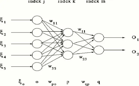
Figure 3 Multi-Layer Artificial Neural Networks.
3.
BACK-PROPAGATION ALGORITHM
Back-propagation algorithm [11] consists of two phases. First phase is the forward phase. This is the phase where the activations propagate from the input layer to the output layer. The second phase is the backward phase. This is the phase where then the observed actual value and the requested nominal value in the output layer are propagated backwards so it can modify the weights and bias values. The following figure 4 is an example of the forward propagation and backward propagation.
Figure 4 Forward and Backward propagation.
In forward propagation, the weights of the needed receptive connections of neuron j are in one row of the weight matrix. In backward propagation, the neuron j in the output layer calculates the error between the expected nominal targets. The error is propagated backwards to the previous hidden layer and the neuron i in the hidden layer calculates this error that is propagated backwards to its previous layer. This is why the column of the weight matrix is used. n the actual output values. This output value is known from both the forward propagation and backward propagation.
Step 0: Initialize weights. (Set to small random values).
Step 1: While stopping condition is false, do Steps 2-9,
Volume 2, Issue 1, January 2013
Page 78
Step 3: Each input unit (Xi, i= 1, . . . . , n ) receives input signal xi and broadcasts this signal to all units in the layer
above (the hidden units).
Step 4: Each hidden unit (Zj, j= 1 . . . p) sums its weighted inout signals,
applies its activation function to compute its output signal,
zj = f(z_inj ),
and sends this signal to all units in the layer above (output units).
Step 5: Each output unit (Yk, k = 1 . . . m) sums its weighted input signals,
and applies its activation function to compute its output signal,
yk = f(y_ink).
Back propagation of error:
Step 6: Each output unit (Yk, k = 1 . . . m) receives a target pattern corresponding to the input training pattern,
computes its error information term,
k = (tk - yk)f’(y_ink ),
calculates its weight correction term (used to update wjk later),
wjk = k zj
calculates its bias correction term (used to update wok later),
wok = k
and sends k to units in the layer below.
Step 7: Each hidden unit (Zj, j = 1, . . . . , p) sums its delta inputs (from units in the layer above),
multiplies by the derivative of its activation function to calculate its error information term,
j = _inj f’(z_inj),
calculates its weight correction term (used to update vij later),
vij = j xi,
and calculates its bias correction tern (used to update voj later), voj = j
Update weights and biases:
Step 8: Each output unit (Yk, k = 1 . . . m) updates its bias and weights (j = 0 . . . p):
wjk(new) = wjk(old) + wjk,
Each hidden unit (Zj, j = 1 . . . p) updates its bias and weights (i = 0 . . . n):
Volume 2, Issue 1, January 2013
Page 79
Step 9: Test stopping condition.
4.
PARTICLE SWARM OPTIMIZATION
Problem solving is a population-wide phenomenon, emerging from the individual behaviors of the particles through their interactions. In any case, populations are organized according to some sort of communication structure or topology, often thought of as a social network.
In PSO, each particle keeps track of its coordinates in the solution space which are associated with the best solution (fitness) that has achieved so far by that particle. This value is called personal best, pbest.
Another best value that is tracked by the PSO is the best value obtained so far by any particle in the neighborhood of that particle. This value is called gbest.
In PSO each particle tries to modify its position using the following information:
The current positions,
The current velocities,
The distance between the current position and pbest,
The distance between the current position and the gbest.
The modification of the particle‘s position can be mathematically modeled according the following equation:
Vi k+1 = wVik +c1*rand1 ( )*(pbesti-sik) + c2 *rand2 ( )* (gbest- sik) (1)
where, Vik : velocity of agent i at iteration k, w : weighting function,
cj : weighting factor for j=1,2.
Rand : uniformly distributed random number between 0 and 1, sik : current position of agent i at iteration k,
pbesti : pbest of agent i, gbest : gbest of the group.
The following weighting function is utilized in (1).
w = wMax-[(wMax-wMin)iter] / maxIter (2)
where, wMax = initial weight, wMin = final weight,
maxIter = maximum iteration number, iter =current iteration number.
The current position (searching point in the solution space) can be modified by the following equation:
Sik+1 = sik + Vik+1 (3)
5.
HYBRID PSO-BP ALGORITHM
The PSO-BP is an optimization algorithm combining the PSO with the BP [7] [8]. Similar to the GA; the PSO algorithm is a global algorithm, which has a strong ability to find global optimistic result, this PSO algorithm, however, has a disadvantage that the search around global optimum is very slow. The BP algorithm, on the contrary, has a strong ability to find local optimistic result, but its ability to find the global optimistic result is weak. By combining PSO with the BP, a new algorithm referred to as PSO-BP hybrid algorithm is formulated in this paper.
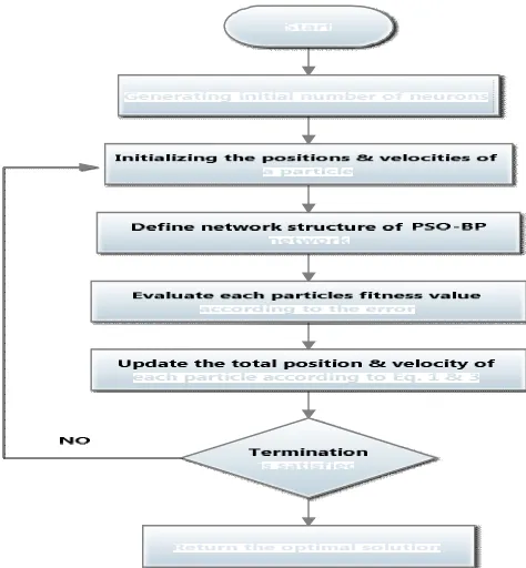
The PSO–BP algorithm can be summarized as follows:
Step 1: Initialize the positions (weight and bias) and velocities of a group of particles randomly.
Step 2: The PSO-BP is trained using the initial particles position.
Step 3: The learning error produced from BP neural network can be treated as particles fitness value according to
initial weight and bias.
Step 4: The learning error at current epoch will be reduced by changing the particles position, which will update the
weight and bias of the network.
Volume 2, Issue 1, January 2013
Page 80
(ii) The “gbest” value (lowest learning error found in entire learning process so far) are applied to the velocity update equation (Eq. 1) to produce a value for positions adjustment to the best solution or targeted learning error.
Step 5: The new sets of positions (NN weight and bias) are produced by adding the calculated velocity value to the
current position value using movement equation (Eq. 1). Then, the new sets of positions are used to produce new learning error in feed-forward NN.
Step 6: This process is repeated until the stopping conditions either minimum learning error or maximum number of
iteration are met.
Step 7: The optimization output, which is the solution for the optimization.
Figure 5 Hybrid PSO-BP Learning Process
Figure 6 Flowchart for Hybrid PSO-BP Algorithm.
6.
RESULTS
Volume 2, Issue 1, January 2013
Page 81
To set up the handwriting recognizer follows the steps below i. Click the Handwriting Recognizer Button.
ii. Select the input image by clicking the ‘select’ button and choosing the image using the dialogue shown. iii. Click the “Trace Characters” button
iv. Once completed results will be shown in output log.
7.
CONCLUSION
We proposed an efficient Hybrid Particle Swarm Optimization and Back propagation algorithm to enhance the performance of Artificial Neural Network for Hand Writing Recognition by means of optimizing ANN weights. Finding a more relevant fitness function or using a type of discriminative training may also improve the results and achieve superior performance than any other Hand Written Recognition methods existed before.
REFERENCES
[1] Kuok King Kuok., Sobri Harun., Siti Mariyam Shamsuddin.,’’ Particle Swarm Optimization Feedforward Neural Network for Hourly Rainfallrunoff Modeling in Bedup Basin, Malaysia’.
[2] Rita Yadav, Danvir Mandal, 2011,’’ Optimization of Artificial Neural Network for Speaker Recognition using Particle Swarm Optimization’’
[3] Buffa F., Porceddu I. 1997”Temperature forecast and dome seeing minimization. A case study using neural network model‘, http://www.pd.astro.it/TNG/TechRep/rep67/rep67.html
[4] Claus, D.”Handwritten Digit Recognition‘, http://www.robots.ox.ac.uk/~dclaus
[5] Malothu Nagun, N Vijay Shankar Annapurna,’ 2011,’’ A novel method for Handwritten Digit Recognition with Neural Networks’’
[6] Mahamed G. H. Omran, 2004,”Particle Swarm Optimization Methods for Pattern Recognition and Image Processing”
[7] Jing-Ru Zhang, Jun Zhang, Tat-Ming Lok, Michael R. Lyu, 2006,” A hybrid particle swarm optimization–back-propagation algorithm for feedforward neural network training”
[8] H. Shayeghi, H.A. Shayanfar, G. Azimi, 2010,’’ A Hybrid Particle Swarm Optimization Back Propagation Algorithm for Short Term Load Forecasting”
[9] Keysers D., NeyH, Paredes R., Vidal E. 2002,”Combination of Tangent Vectors and Local Representations for Handwritten Digit Recognition’’
[10] Jonathan Mooney, 2008,’’ A Character Recognition Artificial Neural Network”
[11] Nearest Neighbor Rule: A Short Tutorial. 1995,