DEMOGRAPHIC RESEARCH
VOLUME 31, ARTICLE 11, PAGES 275
−
318
PUBLISHED 29 JULY 2014
http://www.demographic-research.org/Volumes/Vol31/11/ DOI: 10.4054/DemRes.2014.31.11
Research Article
A method for socially evaluating the effects of
long-run demographic paths on living standards
Nick Parr
Ross Guest
©2014 Nick Parr and Ross Guest.
This open-access work is published under the terms of the Creative Commons Attribution NonCommercial License 2.0 Germany, which permits use, reproduction & distribution in any medium for non-commercial purposes, provided the original author(s) and source are given credit.
2 Social valuation of demographic paths 278 2.1 The effect of population age structure on living standards 278
2.2 Valuing population trends 279
2.3 Comparing social values of alternative demographic paths 281
3 Simulations 283
3.1 Projections of the support ratio Lt/Nt 285
3.1.1 Baseline series 285
3.1.2 The effect of projected mortality decline 285 3.1.3 The effects of future net immigration 287
3.1.4 The effects of future fertility 289
3.2 Social valuations of projections of the support ratio Lt/Nt 290
3.2.1 Introduction 290
3.2.2 The effect of projected mortality change on social valuations 291 3.2.3 The effects of future migration on social valuations 293 3.2.4 The effects of future fertility on social valuations 294 3.2.5 The effect of extrapolated changes in labour force participation on
social valuations
295 3.2.6 The effect of weighting for consumption needs 297 3.2.7 The effect of diminishing returns to scale on the valuations 298 3.2.8 The effect of aversion to intergenerational inequality on social
valuations
301
4 Discussion and conclusion 303
5 Acknowledgements 307
References 308
Appendix A 314
A method for socially evaluating the effects of
long-run demographic paths on living standards
Nick Parr1
Ross Guest2
Abstract
BACKGROUND
The paper is motivated by the need for improved social evaluation of prospective demographic change in order to better inform policies that are designed to reduce the very long-run costs of population ageing and to achieve sustainable economic development.
OBJECTIVE
What is the very long-run social value of a given demographic path? What is the value of changes in mortality, immigration, fertility, and labour force participation? How important are shorter-term demographic changes relative to very long-term effects in determining the social value of the demographic path?
METHODS
A new simulation method is applied for socially evaluating demographic paths, by separating a demographic path into a stable population component and a transition path component. Sensitivity analyses are conducted with respect to demographic assumptions, labour force participation assumptions, and consumption needs by age, returns to scale, and intergenerational value judgements.
RESULTS
The application to Australia shows the considerable social cost, in terms of the loss of discounted consumption per capita, of improvements in mortality and gains from higher immigration and increased participation. The effect of fertility, however, is very sensitive to assumptions about the age-specific consumption needs of the population and social value judgements about intergenerational equity.
CONCLUSIONS
Our method socially evaluates the very long-run implications of specified constant fertility, mortality, and migration, giving consideration to both the transition path and the ultimate stable state. Mortality improvement is costly and higher immigration is beneficial. The impact of higher fertility is sensitive to assumptions about consumption needs and intergenerational equity.
1. Introduction
This paper proposes a method for socially evaluating the trajectories of long-run population projections. Governments in developed countries have, in recent decades, become increasingly concerned about the future population ageing that is reflected in their population projections, and which has implications for national prosperity,
government budgets3, and sustainable economic development. A range of public
policies have been introduced to either slow down population ageing or to ameliorate its effects on national prosperity and government budgets. Policies to slow down ageing include pro-fertility policies such as child subsidies of various kinds (McDonald 2006; Gauthier 2007; Guest and Parr 2010; Parr and Guest 2011; Guest and Parr 2013) and pro-immigration policies (Malmberg 2006). Policies to boost both supply and demand
for older workers (OECD 2006)4 are designed to reduce the national economic burden
of ageing. Population is also seen as a mediating factor in sustainable economic development. The Australian Government, for example, produced a Sustainable Population Strategy in 2011 (Commonwealth of Australia 2011). Such strategies, however, typically sidestep any social evaluation of the nation’s prospective demographic path, and rather focus on the implications of demographic paths for the ‘needs’ of the population in terms of infrastructure such as water, energy, transport and communication, of government services, education, and training, and of environmental amenity.
It is the public policy attention to the economic effects of demographic change that motivates the social evaluation of alternative demographic paths proposed in this paper.
3 Popular discussion of the costs of population ageing tends to conflate the national economic burden of
ageing with the fiscal costs of ageing. The former refers to the effect of ageing on national consumption per capita over time, while the latter refers to the expected impact on government revenue and spending.
4 The OECD is currently (mid 2011 to 2014) conducting a follow up review of its major report: Live Longer,
Work Longer: A synthesis report, which surveys the policy initiatives that have been taken, and are planned to be taken, to boost the employment of older workers. http://www.oecd.org/employment/employment
The standard approach taken to such evaluations in the population economics literature is to embed demographic structure into an intertemporal macroeconomic model of optimal economic growth and then simulate the long-run effects of demographic
change. The seminal study is Cutler et al. (1990), which has spawned a large literature5.
A key feature of these models is optimising behaviour of either individual agents or a social planner. Much controversy exists in the literature about the merits of such an approach. For a comprehensive, accessible critique of representative agent models see
Kirman (1992); and for a post-GFC6 critique that includes the more sophisticated
version known as dynamic stochastic general equilibrium (DSGE) models see Quiggin (2012). In Cutler et al. (1990), for example, a social planner maximises a social welfare
function, which is a discounted utility function7, over an infinite time horizon. Aside
from any issues about the economic assumptions in their model, their method does not consider the full long-run effects of demographic change. Their population projection is
truncated after a finite period of time8, beyond which the age structure remains constant
at the level existing at the end point of the projected period. It therefore ignores the effect that the momentum of demographic change, created during and preceding the projection period, will have on the age structure in the very long run. In particular, any change to the age and sex composition of a population that affects its reproductive capacity will have long-run ‘echo’ effects on the age composition which reverberate ad infinitum (Auerbach and Kotlikoff 1987). Hence a social evaluation of alternative scenarios for fertility, mortality, and migration should consider the very long-run paths of the resultant population age structure and the terminal stable population to which the
populations converge9. Auerbach and Kotlikoff (1987, 1992) simulate the effects of
projected population age structure on a range of macroeconomic outcomes, including savings rates, wage rates, interest rates, and taxation rates, both for the terminal (long-run”) stable populations and for the more immediate years of the transition towards these outcomes, but do not unify these effects within single figure summary measures of the value of these differences across the full duration of the transition. Moreover, they do not consider examples involving pairs of demographic paths which approach differing terminal stable populations.
In this paper the contribution of the method for socially evaluating long-run population projections is twofold. First, it unifies in a single measure the evaluation of
5 For a recent example see Prettner (2013) and the references therein. 6 Global Financial Crisis of 2008-2009.
7 In Cutler et al. (1990) utility at time t is a CES (constant elasticity of substitution) function of per capita
consumption at time t. This utility for t=0,..,∞ is then discounted to time 0 and summed over the infinite
horizon to give the value of social welfare.
8 They use the (US) Social Security Administration Forecasts for 1990–2065.
the stable populations to which populations converge with the evaluation of the transition paths towards these asymptotes. This is done by partitioning the social value into a stable population component and a transition path component. Second, it allows the long-run momentum effects of changes in fertility, mortality, and migration over a
finite period to be incorporated into the valuations10. The method also avoids the
controversy over optimising behaviour by specifying an exogenous path for consumption per capita that is perturbed mechanistically by shifts in the employment to population ratio, which are in turn determined by demographic change. The approach
does, however, incorporate value judgements of a ‘social planner’11 – in particular,
trade-offs between the welfare of generations in the present and future, which imply
judgements about intergenerational equity12. Such trade-offs are implicit in any
assessment of the role of population as a mediating factor in sustainable development. The model here adopts typical values of the key parameters driving the intergenerational distribution of living standards – that is, the social rate of time preference and social aversion to intergenerational inequality.
Section 2 of the paper describes this new methodology in its simplest form. More complex variants of the methodology are presented in Appendices A and B. In Section 3 the method is applied to prospective demographic paths for Australia, illustrating the sensitivity of the results to mortality, migration, and fertility parameters. Section 3.1 describes the demographic projections and the associated employment-to-population ratios, and Section 3.2 discusses the results of valuations of the differences between these demographic paths. The final section (4) concludes the paper.
2. Social valuation of demographic paths
2.1 The effect of population age structure on living standards
Living standards are defined here in material terms only, in particular as national consumption per capita. The following framework is useful for illustrating the important implications of the population age distribution for living standards:
10 These momentum effects would manifest over an infinitely long time horizon.
11 The ‘social planner’ is a theoretical concept, of course. It may also be thought of as a benevolent dictator,
government, or even the enfranchised citizen.
12 This literature has a long pedigree in optimal saving models, Ramsey (1928) being the seminal
t t
t t
t t
t t
N L L Y Y C N
C = (1)
The symbols in this identity refer to the following national aggregates: Ct is
consumption of goods and services at time t, Nt is the effective number of consumers
(either total population or a needs-weighted population e.g. as defined by Cutler et al.
1990 or Guest and McDonald 2001), Yt is output of goods and services (gross domestic
product, GDP), and Lt is employment (for example, total hours worked). The ratio Ct/Nt
is consumption per effective consumer, Ct/Yt is the consumption share of GDP, Yt/Lt is
average labour productivity, and Lt/Nt is the employment to population ratio or support
ratio13.
Equation (1) can be re-expressed using age-specific components:
t t x
t x
t x
x xt
t t
t t
t t
N N N E H L Y Y C N
C ,
, , ,
∑
= (2)
where Hx,t denotes hours worked per employed person in age and sex group x at time t,
and hence =∑
x xt xt t
x H E
L, , , where Ex,t is the number of employed persons in age and
sex group x, and Nx,t is population in age and sex group x. In (2) the population age
structure affects living standards through the age-specific variation in Hx,t and Ex,t/Nx,t.
2.2 Valuing population trends
Assumptions can be made about the way in which demographic changes affect Ct/Yt and
Yt/Lt: see Cutler et al. (1990), and for a more recent empirical analysis for OECD
countries using a similar framework to that in (1) see Guest (2007). This framework, however, requires a range of assumptions about the economic structure and behaviour of consumers and firms, which are deliberately avoided in this paper. Here the aim is to
isolate the role of Lt/Nt, which is achieved through two simplifying assumptions. First,
the simplest form of economy is adopted: an economy with no net exports and no
investment, implying Ct= Yt. Second, output (Y) is determined by a simple production
function (without capital):14
13 For discussion of the economic implications of (zero migration) stable age distributions see Arthur and
McNicoll (1978) and Lee (1980).
14 We are grateful to an anonymous referee for pointing out the need to specify a production function in which
α
t t
t AL
Y = (3)
where At = A0(1 + gA)t is a labour-augmenting technology variable growing at a
constant rate gA which is independent of the age composition of the population, and α is
the returns-to-scale parameter15.
Hence the path of living standards for future values of t can be written (substituting
(3) into (1) and simplifying):
(
)
t t t A t t N L g Y C N C α + = 1 0 0 (4)Given that Lt and Nt are both exogenous, given by demographic data, the path of
living standards is also exogenous. Alternative paths of living standards can be evaluated by specifying an objective function:
(
)
∑
∞ = − + = 0 1 t t t t N C fV ρ (5)
where ρ is a social discount rate (discussed below). The function
t t N C
f captures the
social weighting of
t t N C
f and can take various functional forms. Here we take the
simplest possible form:
= t t t t N C N C
f . Appendix A discusses a common alternative
functional form in the literature and introduces a parameter that captures the social
aversion to intertemporal inequality in
t t N
C , and simulations are reported for non-zero
values. In the simplest case where this parameter is zero the objective function is:
+ + =
∑
∞ = t t t t A N L g Y C V α ρ 0 0 0 1 1 (6)From (6), the social evaluation of alternative paths for living standards depends on
the path of t t
N Lα
and the factor
t A
g
+ +
ρ
1
1 . The choice of a value for ρ depends on
judgements about the social value of the consumption of present relative to future generations (Samuelson 1958). Some authors have argued that any value of ρ greater than zero is unethical since it implies that the welfare of future generations is less important simply because they live in the future rather than the present (Ramsey 1928; Pigou 1932). Others favour a positive value of ρ by appealing to uncertainty about the future of the world (Stern 2007) and/or to the observed saving rates of individuals
(Weitzman 2007)16. Typical values for ρ found in the literature range from 0.001 to
0.02 (as surveyed in Scarborough 2011). The value adopted here is 0.017517.
The purpose of the simulations, discussed below, is to assess the role of demographic assumptions in generating
t t
N Lα
and hence V, and the sensitivity of these
results to alternative values of key parameters gA, ρ and a parameter that captures social
aversion to inequality in intertemporal consumption (discussed in Appendix A). Appendix B shows that the valuation function (6) is readily extended to accommodate
linear effects of the projected proportionate age distributions of the population on (Yt/Lt)
or (Ct/Yt).
2.3 Comparing social values of alternative demographic paths
The method we propose applies to projections in which Ltα/Nt converges in the very
long run to a constant value. The focus in this paper is on the subclass of population projections in which age-specific fertility, age-specific mortality rates, and the annual number and age distribution of immigration all eventually reach constant levels. Under these conditions the population asymptotically approaches a stable age distribution and, if fertility is below replacement level and net immigration is inwards, a stationary population (Pollard 1973; Espenshade et al. 1982). Attention is further restricted to
projections where the age-specific labour force participation rates (Hx,t Ex,t/Nx,t in (2))
also eventually become constant. Thus the valuations are of the very long-run implications of finite changes to population age structure and labour force participation.
16 Individuals tend to be myopic in their own life planning in well-known ways that indicate a rate of time
preference. As an example of a form of myopia in an intergenerational context, a mother is likely to care more about her children than her grandchildren and even less about her great grandchildren.
Ct/Ntcan be decomposed as follows: − + = s s t t s s t t N C N C N C N C (7)
where (Cs/Ns) is a constant which equals the living standard for the asymptotic
(henceforth “terminal”) stable age distribution of the projection series. Substituting from (7) into (6):
− + + + + + =
∑
∑
∞ = ∞=0 0
0 0 1 1 1 1 t s s t t t A t s s t A N L N L g N L g Y C
V α α α
ρ
ρ (8)
In (8) the value of the series is expressed as two components: the first is the value of the terminal stable population and the second a value of the difference between the projection series and the terminal stable population. We term the first of these the “(terminal) stable population component” and the second component the “transition path component”. Hence the difference in social values of any two demographic projections, A and B, can be expressed as the sum of a “difference in stable population components” plus a “difference in the transition path components”.
− − − + + + − + + = −
∑
∑
∞ = ∞ = 0 , , , , , , , , 0 , , , , 0 0 1 1 1 1 ) ( ) (t sB
B s B t B t A s A s A t A t t A
t sB
B s A s A s t A N L N L N L N L g N L N L g Y C B V A V α α α α α α ρ ρ (9) ) ( )
(A V B
V − is finite when ρ>gA, in which case the value of the stable
population component in (7) is simply calculated as the sum of a geometric series18.
The elements of the transition path component can be calculated for all values of t for
which the projection has been calculated. The residual element may be estimated
18 We consider the case of discrete (annual) population change as opposed to continuous change. Under
through model-based imputation19. Equations (8) and (9) may be modified to
incorporate linear effects of the projected proportionate age distributions of the population on (Yt/Lt), (Ct/Yt) or (Ct/Lt) (see Appendix B).
Cumulative contributions to the differences in value for various future intervals of time, both in absolute terms and in proportionate terms, may also be calculated. The
contribution to the difference in value for the first T years of the projection is:
− + + = −
∑
= = = Tt tB
B t A t A t t A T t T t N L N L g Y C B V A V 0 , , , , 0 0 0
0( ) ( ) 11
α α
ρ (10)
This can be converted into proportionate terms by dividing by the (total) value of the difference from (9). Such figures can provide an indication of the inadequacy which valuations considering only trends over these finite periods of time would have.
3. Simulations
The simulations give social valuations of differences in demographic projections for Australia. A baseline series is compared with a range of variants, each of which differs from the baseline in only one of the assumptions for future mortality, migration, and
fertility20. The valuations use a rate of labour-augmenting productivity growth (g
A) of
1.5% per annum, a returns to scale parameter of 1.0,21 and a social discount rate of
1.75% per annum. As extensions, consumption units per effective person are calculated by weighting the consumption needs of the population by age, following, firstly, Cutler et al. (1990) and, secondly, weights proposed for Australia by Guest and McDonald (2001). Under Cutler et al.’s weights each person aged 0-19 years is given a consumption-needs weight of 0.72 and each person above age 65 is given a weight of 1.27. The weights proposed by Guest and McDonald (2001) are for narrower age bands.
19 The mathematical function used for this must tend to zero as time tends to infinity. The value of this
element is estimated through either summation of a series or integration of a curve.
20 Theoretically the valuations will be affected also by the proportional age structure of the start population,
and hence by past fertility, mortality, and migration. We omit to illustrate the sensitivity of results to this distribution.
21 Constant returns to scale is adopted here in order to avoid the deflating of future labour implicit in the term
α
L with α<1. This could have been avoided by introducing capital into the production function (3), which
The consumption weight is lowest for 0-15 year olds (0.68) and highest for the 75 and over age group (1.19). There are small undulations in the values between these age
ranges22. We also consider the effect of returns-to-scale parameter (α) of 0.95. A further
extension is to incorporate a parameter for aversion to intergenerational inequality of living standards (Appendix A). All projections use the 2011 estimated resident population of Australia as the base population.
The baseline series illustrates the effects of mortality improving to 2050, as projected by Li (2013) using the Poison Common Factor variant of the Lee-Carter
model, and remaining constant thereafter23. In addition, the levels and age distributions
of both fertility (TFR = 1.9) and net international migration (180,000 per annum) are assumed to remain constant at roughly the levels for recent years (ABS 2012a, 2013a). The age- and sex-specific labour force participation rates are assumed to remain constant at the 2011 levels (ABS, 2012b). Table 1 summarises the assumptions for the baseline series and the differences between the variant series and the baseline. Section
3.1 describes the projected trajectories for hours worked per head of population (Lt/Nt)
(Section 3.1) followed by the projected social valuations (Section 3.2).
22 Data which allow consumption weights to be developed for a range of countries (excluding Australia) are
available from the National Transfer Accounts project (http://www.ntaccounts.org).
23 The plausibility of an upper limit to life expectancy has been debated in the literature (Oeppen and Vaupel
Table 1: Specification of the baseline and variant series Series Assumptionsa
Baseline Life expectancy increases to 87.6 for males and 90.7 for females by 2050 using the projection of Li (2013), and is constant thereafter.
Net migration constant at 180,000 per annum. Total Fertility Rate constant at 1.9.
L b F P ti i ti t t t 2011 l l A Mortality constant at 2011 levels
B Net migration constant at 90,000 from 2011 onwards. C Net migration constant at 270,000 from 2011 onwards D Net migration constant at zero from 2011 onwards E Total Fertility Rate constant at 1.7 from 2011 onwards F Total Fertility Rate constant at 2.1 from 2011 onwards
Note: a. For the variant series all assumptions other than the tabulated are as per the baseline series.
3.1 Projections of the support ratio Lt/Nt
3.1.1 Baseline series
Under the baseline series the population of Australia is projected to increase with a
decreasing growth rate, and to age significantly24. The hours-worked-to-population
ratio (Lt/Nt) is projected to decrease at a progressively more gradual rate, from 16.6 in
2011 to 15.0 in 2050, 14.7 in 2100, 14.5 in 2200, and 14.0 in the terminal stationary population (Figure 1). The population is projected to increase from 22.3 million in 2011 to 35.6 million by 2050, 50.1 million by 2100, 73.0 million by 2200, and towards 153.4 million in its terminal stationary state.
3.1.2 The effect of projected mortality decline
Under series A, which differs from the baseline series only in its assumption of constant
mortality, the projected reduction in Lt/Nt is smaller than under the baseline, reaching
24The population increases under the baseline projection even though fertility is below replacement. This is
15.4 for 2050, 15.3 for 2100, and 15.0 in the terminal stationary population (Figure 1). The difference from the baseline is due to the lower projected percentages of the population in the low-participation-rate-older-ages under the constant mortality (series A) scenario, compared to the baseline scenario with its projected mortality improvement. Comparison of this constant mortality variant series with the baseline
shows that only 26.4% of the projected reduction in Lt/Nt by 2050, 31.1% of the
projected reduction to 2100, and 37.4% of the projected change to the terminal stationary population are attributable to the projected improvements in mortality. Even though in the baseline scenario mortality improvement ceases abruptly in 2050, the
widening gap in Lt/Nt post-2050 shows there is a significant longer-term flow-on effect
of the projected improvement in mortality between 2011 and 2050 over the post-2050 period, which illustrates the limitation in truncating the projection period too early.
Under constant mortality the projected population growth is less than under the baseline: the population is projected to reach 34.0 million in 2050, 66.9 million in 2200, and 120.1 million in the terminal stationary population.
Figure 1: Effects of varying mortality on projected support ratio (Lt/Nt):
Baseline forecast of mortality improvement vs constant mortality at 2011 level
13 13.5 14 14.5 15 15.5 16 16.5 17
2011 2031 2051 2071 2091 2111 2131 2151 2171 2191
L/N
Year
Constant Mortality
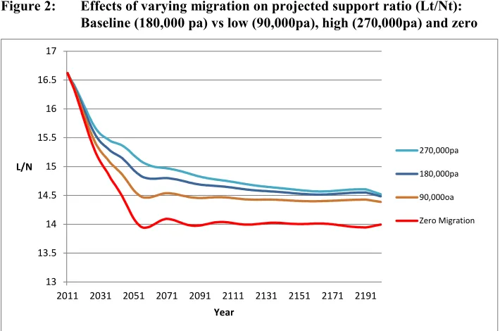
3.1.3 The effects of future net immigration
The contrasts between series B (a reduction in net migration to 90,000) and series C (an increase to 270,000) from the baseline show that in the short and medium term the
higher the level of immigration the higher the Lt/Nt (Figure 2) (Bloom et al. 2010;
McDonald and Temple 2010). There are, however, diminishing returns to increasing net migration: the effects on this ratio of an increase in net migration from 180,000 to 270,000 per annum are slightly smaller than those of an increase from 90,000 to 180,000. In the very long run the effects of higher or lower net migration approach zero25, 26, 27. Under all plausible scenarios, immigration does not arrest the decline in Lt/Nt due to population ageing28.
The effect of higher net immigration on Lt/Nt increases gradually until about
205429, and decreases gradually thereafter. The terminal stationary populations for all
the series with non-zero migration are identical in their proportionate age structures and hence hours-worked-to-population ratios.
Under series D (zero net migration) the reduction in Lt/Nt in the absence of net
migration is steeper than under all three positive net migration scenarios, falling to 14.1 in 2050 and 14.0 in 2100. The difference from the baseline series rises to a maximum in
25 The equality of the proportionate age distributions of the terminal stationary populations, and hence of
support ratios, is the product of the assumed equal proportionate age distributions of these migrant intakes. If the higher and lower variants differed from the baseline in the proportionate age distributions for net migration then differing age structures for the terminal stationary populations would result (Pollard 1973).
26 For simplicity it is assumed the proportionate age and sex distribution of net migration is invariant to its
total level. The recent historical variation in net immigration in Australia has primarily been due to variation in immigration, as opposed to emigration. The age distributions of immigrants and emigrants differ, with the former being slightly younger on average than the latter (ABS 2012c). Hence in practice a higher level of net migration would be expected to have a somewhat younger profile and a lower level a somewhat older profile.
27 The model assumes labour force participation rates and labour productivity are invariant to the level of
immigration. In contrast to most other OECD countries, in Australia the unemployment rate for the migrant population differs little from that for the native-born. The labour force participation rate for migrants is slightly below that for the Australia-born. The percentage of the employed working part-time is lower for the overseas-born than for the Australia-born, particularly for females (Massey and Parr 2012; DIAC 2013). There may also be positive or negative ‘spillover effects’ of the level of immigration on the employment levels of the native-born. However, the international literature suggests such effects are generally minor (Kerr and Kerr 2011). The economic outcomes of the children of immigrants also differ from those of the native-born (DIAC 2013).
28 Net migration of well over 800,000 per annum would be needed to maintain L
t/Nt at around its 2011 level. Even with such levels of migration the ratio would decline from around 2045 onwards.
29 The maximum difference between the 270,000 per annum net migration projection and the 180,000 per
2055 and thereafter decreases. Under zero migration the terminal stable age
distribution differs from that for positive net immigration, with Lt/Nt (13.8 hours
worked per week per capita) being appreciably lower.
The projected population under the high migration (270,000 per annum) rises to 40.7 million by 2050, 100.7 million by 2200, and 230.1 million in the terminal stationary state.
Figure 2: Effects of varying migration on projected support ratio (Lt/Nt): Baseline (180,000 pa) vs low (90,000pa), high (270,000pa) and zero
Under the low migration variant (90,000 per annum) the projected population growth is considerably less: the population reaches 30.5 million in 2050, 45.4 million in 2200, and 76.7 million in the terminal stationary state. Under zero migration the projected population rises gradually to a peak of 25.4 million in 2051 before declining gradually to 17.7 million by 2200 and towards zero asymptotically. The sizes of the projected terminal stationary populations are in direct proportion to the size of the migrant intakes (Pollard, 1973; Espenshade et al. 1982; Schmertmann 1992, 2012).
13 13.5 14 14.5 15 15.5 16 16.5 17
2011 2031 2051 2071 2091 2111 2131 2151 2171 2191
L/N
Year
270,000pa
180,000pa
90,000oa
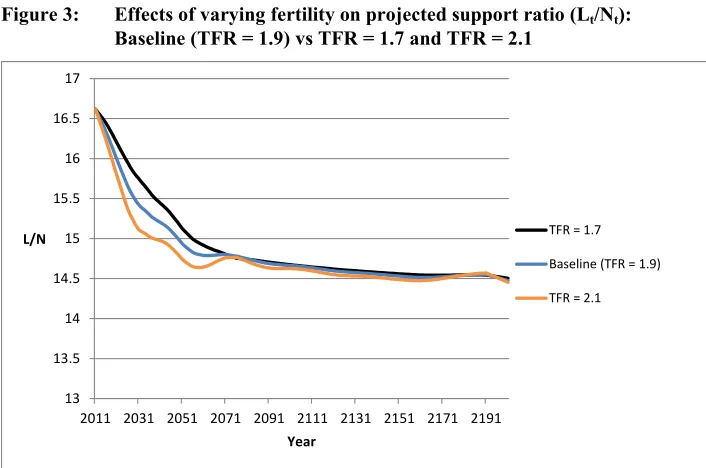
3.1.4 The effects of future fertility
Under the lower fertility (TFR = 1.7) projection Lt/Nt is significantly higher in the short
term than under the baseline, whilst under the higher fertility projection (TFR = 2.1)
Lt/Nt is significantly lower (Figure 3). The differences in Lt/Nt between the baseline and
variant projections increase until they reach their maximum values around 2031, after which point they reduce as the effect of the fertility difference affects the sizes of above-average hours worked per person (i.e., over age 20) age groups as well as the
below-average hours worked per person age groups below age 2030. By around 2070
the differences in Lt/Nt between the projections with differing fertility levels are small.
This illustrates the general result that the long-run effects on Lt/Nt of alternative fertility
scenarios are small (Weil 1999). The Lt/Nt for the terminal stable population under the
lower fertility scenario (TFR = 1.7) (14.1 Lt/Nt) is slightly higher than for the baseline
scenario (14.0), whilst that for the higher fertility scenario (TFR = 2.1) is slightly lower
(13.9 hours per week)31, 32. These results reflect a more general pattern of the Lt/Nt for
the terminal stable populations decreasing as fertility increases across the
below-replacement range of values for fertility33, 34. In contrast to the above scenarios with
positive net immigration, when migration is zero a TFR of around 2.35 produces the
highest value of L/N in the terminal stationary population, with the projected mortality
for 2050.
The projected population growth under the low fertility (TFR = 1.7) scenario is slightly less in the short-to-medium run compared to under the baseline, but very considerably less in the very long run. By 2050 the population is projected to be 33.9 million, just 1.7 million less than the baseline. However, by 2200 it is projected to be 54.3 million (18.7 million or 25.6% less) and the terminal stationary population of 67.5
million is less than half (only 44.0%) of that for the baseline series30. Under the high
fertility scenario (TFR = 2.1) the population is projected to grow to 37.4 million by
30 The maximum difference in the Lt/Nt between the lower fertility (TFR = 1.7) scenario and the baseline
scenario is 0.33 hours per week per capita, whilst that between the higher fertility scenario and the baseline is 0.31 hours per week per capita. Both maxima are reached in 2031.
31 Under a TFR = 0 assumption the Lt/Nt in the terminal stable population is 15.65. With decreasing fertility
(below replacement level) the proportion of the terminal stationary population who are former immigrants increases and as fertility approaches zero the Lt/Nt approaches that of the surviving immigrant population.
32 In age distribution of the terminal stable population under a TFR of 2.1 numbers decrease monotonically
with increasing age, in contrast to patterns of increasing numbers up to a maximum at age 49 with a TFR of 1.9 and a maximum at age 52 with a TFR of 1.7.
33 See Schmertmann (1992) for explanation of the variation by the fertility level in the age distributions of
stationary populations with constant immigration.
34 It should be noted that the value of hours worked per person in the terminal stable population increases
2050 and to 99.3 million by 2200. Under this slightly above-replacement level of fertility the population would continue to increase indefinitely at a very gradual rate.
Figure 3: Effects of varying fertility on projected support ratio (Lt/Nt):
Baseline (TFR = 1.9) vs TFR = 1.7 and TFR = 2.1
3.2 Social valuations of projections of the support ratio Lt/Nt
3.2.1 Introduction
The differences in social value between the variant series and the baseline series are calculated using (9). The “Terminal Stable Population” and “Transition Path” components of this difference are also given (9). The differences in social value are also expressed as percentages of the social value of the baseline projection and as a
percentage of the 2011 social value of Lt/Nt. Table 2 summarises the results. We then
illustrate the changes to the effects of future mortality, migration, and fertility under an alternative trajectory for labour force participation (Table 3), under two different weightings of the population for consumption needs (Table 4) and diminishing returns to scale (Table 5). Finally, the effects of introducing a degree of aversion to intergenerational inequality are considered (Table 6).
13 13.5 14 14.5 15 15.5 16 16.5 17
2011 2031 2051 2071 2091 2111 2131 2151 2171 2191
L/N
Year
TFR = 1.7
Baseline (TFR = 1.9)
Table 2: Differences in components of social value and total social value in units between variant series and baseline series with constant labour force participation rates expressed on a per capita basis:
Australia 2011 onwards
Variant Series Difference from Baseline Seriesa,b Modulus of Difference in Total Valuea Stable
Population Component
Transition Path Component
Total Social
Value Value of As % of Baseline Seriesc
As % of Social Value
in 2011d
A (Constant Mortality) 409.5 -92.1 317.4 5.1 1910.0 B (Net Migration =
90,000) 0.0 -28.0 -28.0 0.5 168.4
C (Net Migration = 270,000)
0.0 16.5 16.5 0.3 99.1
D (Net Migration = 0) -74.2 -79.3 -153.5 2.6 923.8
E (TFR = 1.7) 54.9 -7.9 47.0 0.8 282.9
F (TFR = 2.1) -27.1 -6.5 -33.7 0.6 202.7
Notes: a. Using gA = 1.5% p.a., ρ = 1.75% p.a., α=1, and β = 0.
b. Expressed as a multiple of the 2011 consumption value of one hour worked per week per capita
c. Value of baseline series = 5845.5 times the consumption value of one hour worked per week per capita in 2011. d. As multiple of consumption value of 2011 L/N (16.6 hours worked per week per capita).
3.2.2 The effect of projected mortality change on social valuations
In the constant mortality variant series (series A), the total social value is 5.1% higher
than in the baseline series. This represents the cost35 of the projected improvements in
mortality to 2050 under the baseline series and is primarily due to the greater value of the terminal stable population under the higher mortality (constant) scenario (column 2). The (negative) difference in transition path components reflects the differences between the values of the constant mortality series (A) and the value for its terminal stable population being smaller than the equivalent differences for the baseline series. The 5.1% increase in social value is equivalent to 317.4 times the consumption value of
35 Henceforth we refer to negative differences in values as “cost” and positive differences as “benefits”. It
one hour worked per week per capita in 2011(shown by the “total value” in column 4 of Table 2) and over 19 times the 2011 total consumption, which is a consumption value
of A$830,682 per capita36,37.
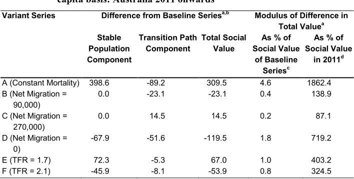
Table 3: Differences in components of social value and total social value in units between variant series and baseline series with extrapolated trend in labour force participation rates by age expressed on a per capita basis: Australia 2011 onwards
Variant Series Difference from Baseline Seriesa,b Modulus of Difference in Total Valuea Stable
Population Component
Transition Path
Component Total Social Value Social Value As % of of Baseline
Seriesc
As % of Social Value
in 2011d
A (Constant Mortality) 398.6 -89.2 309.5 4.6 1862.4 B (Net Migration =
90,000)
0.0 -23.1 -23.1 0.4 138.9
C (Net Migration =
270,000) 0.0 14.5 14.5 0.2 87.1
D (Net Migration =
0) -67.9 -51.6 -119.5 1.8 719.2
E (TFR = 1.7) 72.3 -5.3 67.0 1.0 403.2 F (TFR = 2.1) -45.9 -8.1 -53.9 0.8 324.5
Notes: a. Using gA= 1.5% p.a., ρ = 1.75% p.a., α=1, and β = 0.
b. Expressed as a multiple of the 2011 consumption value of one hour worked per week per capita.
c. Value of baseline series = 6476.1 times the consumption value of one hour worked per week per capita in 2011. d. As multiple of consumption value of 2011 L/N (16.6 hours worked per week per capita).
Another way of interpreting the percentage difference in value is that an immediate and sustained increase in labour force participation in all age and sex groups equivalent to 5.1% of the 2011 level would be required to offset the negative effect on social value of the forecast mortality change between 2011 and 2050. Using (10), the contributions of different time periods to this difference in values can be calculated. Only 2% of the difference in social value is realised over the period 2011-2050 and only 9.6% by 2100. These figures provide an indication of the limitation in truncating the projection period,
36 At the initial time point of the projection (30th June 2011) one Australian dollar officially exchanged for
1.10US$ and 0.77 Euros (Australian Taxation Office 2012).
37This figure is based on an estimated GDP for 2011 of A$1.33 trillion and hence a value of Y
t/Lt of A$3585 per hour worked per week per person. It is based on the strong assumption that the effect of age structure on
and that the cost of the projected mortality improvement is almost entirely the product of assumed very long-run effects.
The estimated total cost of the projected mortality improvement depends on the assumed levels of migration and fertility. Under lower (positive) levels of migration the per capita cost of the projected mortality change is higher, entirely due to a higher Transition Path Component. The greater per capita cost is the product of the concentration of the effect of projected mortality improvement in the older age groups and the generally older transition-path populations that occur under lower migration. Under lower fertility the per capita cost of the projected mortality change is greater than under higher fertility. This is largely accounted for by an increased Stable Population Component, and reflects the generally older age structures with lower fertility. Clearly from (9) the magnitude of the value of any difference in demographic trajectories will be smaller under a higher social discount rate (ρ) than under a lower rate, and larger
under a higher rate of productivity growth (g) compared to under a lower rate.
3.2.3 The effects of future migration on social valuations
Since all the series with positive values of net migration approach the same terminal
stable population21, the differences in social value between these series are entirely due
to the differing transition paths. Table 2 shows that the magnitude of the cost of lowering migration by 90,000 is 28 times the consumption value of one hour worked per week per capita (column 4 of Table 2), which equates to 0.5% of the baseline social value (column 5), whereas the benefit from increasing migration by 90,000 is smaller at 16.5 times the consumption value of one hour worked per week per capita (0.3% of baseline social value). The cost of lowering migration to zero is far larger (2.6% of baseline social value) than that of lowering migration from 180,000 to 90,000. Over half (59.1%) of this larger cost is due to the difference in the values of the terminal stable populations of the non-zero migration and the zero migration projections. Thus whilst the cost in perpetuity of lower migration is very large in absolute terms (for example the cost of a sustained reduction in migration from 180,000 to 90,000 equates to 168.4% of 2011 national consumption (see column 6)), due to the infinitely long duration of this effect, only a very minor increase in labour force participation (0.5% of the 2011 levels), if immediate and sustained, would be needed to counterbalance its effect on the long-run social value.
variations in fertility and in mortality that we consider. This reflects the transitory nature of the effects of such changes in migration levels on the age structure. As a consequence of the earlier pattern of the migration effects, the effects of variations in migration are less sensitive than the effects of variations in fertility or mortality to the
assumed consumption discount rate38.
The estimated valuations of the effects of migration also depend on the fertility and mortality assumptions. With lower, sub-replacement levels of fertility the per capita benefit of higher migration and the cost of lower migration are increased, reflecting the higher proportion of the population who are surviving migrants under lower fertility scenarios. The difference in values between the positive migration projections and the zero migration projections is considerably smaller when fertility is above replacement level, because the “Stable Population Component” is zero at above replacement levels of fertility (the effect of any constant number of migrants tends to become ignorable as the population grows exponentially). Under constant as opposed to improving mortality the per capita effects of variations in net migration between different positive levels are larger.
3.2.4 The effects of future fertility on social valuations
Under positive net migration, projections with lower fertility have higher per capita values than those with higher fertility. The value of series E (TFR = 1.7) is higher than the baseline series by 0.8%, which in turn is 0.6% higher than the value of Series F (TFR = 2.1), and the fertility level which produces the highest value path is zero. For each variant the major component of the differences in social value is the “Stable Population Component” (Table 2).
The effect of any given change in the fertility level is larger under the constant mortality scenario than under the projected mortality improvement of the baseline series, reflecting the generally younger population in the absence of mortality improvement. Moreover, the effects of specified fertility changes on the valuations are smaller at lower, positive levels of migration and larger at higher levels, due entirely to changes in the “Transition Path Component”. This can be explained by the relatively high concentration of the ages of newly arriving migrants in the female reproductive ages. The percentages of the differences in value with the baseline series which are realised by 2050 (17.7% for series E (TFR = 1.7) and 23.9% for series F (2.1)) and by
38The percentages of the differences in value from the baseline for series D (zero migration) are low: just
2100 (22.2% for series E and 34.1% for series F) are larger than those for the mortality variant series and smaller than those for the migration variant series.
The effects of changes in fertility under zero migration differ markedly from those under positive migration. Under zero migration the plot of valuations against the TFR follows an inverted U-shape, with the maximum social value corresponding to a total fertility of 2.25. This TFR is slightly lower than the TFR that maximises the value of the terminal stable population (2.35), due to the increases in the social value of the transition path as fertility reduces. With zero migration the social value of a projection with a TFR constant at 1.7 is 65.3 times the consumption value of one hour worked per week per capita less than that for a projection with a TFR of 1.9, which in turn is 145.4 times the consumption value of one hour worked per week per capita less than the social value for a TFR of 2.1. Under constant mortality at the 2011 level and zero migration the social values of constant fertility which maximise the social value of the projections are lower than those which do so under the projected improvement in
mortality under the baseline scenario39.
3.2.5 The effect of extrapolated changes in labour force participation on social valuations
Sensitivity to age-specific labour force participation rates (LFPRs) is illustrated by an alternative scenario in which the LFPRs are extrapolated over the period between 2011 and 2021 at the linear trend rate of change from 2001 to 2011. The LFPRs remain constant from 2021 onwards. Between 2001 and 2011 LFPRs decreased for age groups below 25 years and increased for all age groups over 30 years, with the largest increases
being in the pre-standard retirement age groups between ages 55 and 65 (Figure 4)40.
Thus the projected age profile for labour force participation is older than the current pattern. Increases in employment to population ratios for females are projected to be considerably greater than those for males, a pattern which was observed between 2001 and 2011. The results are reported in Table 3.
Under the extrapolated labour force participation trends the social values of all
projections are greater than they are under constant patterns of participation41. The
39 See Bloom et al. (2010) for explanation of the relationship between mortality and the optimal fertility for
the share of population of working age in stable populations.
40 Over the period 2010 to 2013 the rates of increase of labour force participation rates above age 55 were
significantly slower than between 2001 and 2010 (ABS 2013b).
41For example, the value of baseline series is 6476.1 times the consumption value of one hour worked per
projected increase in participation produces increases in Lt/Nt up to 2021 under the baseline series, more than offsetting the effects of projected demographic change. A comparison of the results of Table 3 with Table 2 shows that the effects of the projected mortality improvement on the social valuation is smaller under the projected changes to workforce participation than they are under continuation of the current patterns of participation. This is largely the product of the larger projected mortality improvements
being on the older age groups and the effect of this change on Lt/Nt being reduced by
the larger projected increases in the participation rates in the older ages. The effects of changes to migration are also decreased slightly by the projected changes in participation. In contrast, the effects of fertility change on the social valuation are larger under the extrapolated trend for labour force participation rates than under constant participation rates. The increased effect of fertility reflects the growing difference between participation in the under-20 age range and the older age groups, and the greater effects of fertility on proportions of population in the younger ages than on those in the older ages (Bloom et al. 2010).
Figure 4: Employment to population ratios by age and sex: Australia 2001 and 2011
0% 10% 20% 30% 40% 50% 60% 70% 80% 90% 100%
Employment/ Population
Age
3.2.6 The effect of weighting for consumption needs
Weighting for consumption needs using the weights of Cutler et al. (1990) magnifies the effects on the social valuation of changes in proportion of the population aged over 65 years and shrinks the effects of changes in the proportion aged under 20 years. A comparison of Table 4 with Table 2 shows that the effect of the projected mortality improvement is considerably greater on the consumption-weighted valuations than on the unweighted valuation, reflecting the disproportionate effect of the projected mortality change on the older age groups. The effects of changes to net migration are also greater on the valuation relative to the consumption-needs weighted populations than the valuation relative to the unweighted population. The results for the two methods of consumption weighting we consider are similar.
The major difference between the valuations’ relative consumption need-weighted populations and the unweighted populations is in the change of the signs for the effects of fertility. Figure 5 shows that crossovers in the value of hours worked to the (Cutler et al. 1990) consumption-weighted population occur roughly 50 years after the start of the
projection42, 43. Table 4 shows that under the Cutler et al. consumption-needs weighting
the social value of the baseline series (TFR = 1.9) is very slightly greater than that for the low fertility projection (TFR = 1.7), and less than that for the higher fertility projection (TFR = 2.1). Both the signs and the magnitudes of these differences in social value by fertility depend on the assumed trends for mortality and labour force
participation44, and on the consumption-needs weights used and the consumption
discount rate. Further investigation finds a global maximum for the social values of the projections series with the baseline mortality and migration corresponding to a TFR of 3.0745, 46. Under the weighting of Guest and McDonald (2001), both the low fertility
series (TFR = 1.7) and the high fertility series (TFR = 2.1) have a slightly higher value than the baseline.
42 The social value for TFR = 1.7 first falls below the baseline (TFR = 1.9) in 2058, which in turn first falls
below that for TFR = 2.1 in 2061.
43 The contributions of differences in particular years to the difference in social value reflect the effects of
consumption discounting as well as the differences in Lt/Nt. Thus the magnitude of the contributions of future years reduces.
44 Under the increasing labour force participation projection the value of the TFR = 1.7 variant is higher than
that of the baseline series (TFR = 1.9).
45 The global maximum for the value of the terminal stable population occurs when the TFR = 3.25. 46 Under the extrapolated trend for labour force participation the TFR which produces the maximum value is
Table 4: Differences in components of social value and total social value in units between variant series and baseline series with constant labour force participation rates expressed on consumption needs-weighted basis: Australia 2011 onwards
Variant Series Difference from Baseline Seriesa,b Modulus of Difference in Total Valuea Stable
Population Component
Transition Path Component
Total Social
Value Value of As % of Baseline Seriesc
As % of Social Value
in 2011d
Cutler et al. 1990
A (Constant Mortality) 542.0 -117.5 424.5 6.8 2468.1 B (Net Migration =
90,000)
0.0 -40.8 -40.8 0.7 237.0
C (Net Migration =
270,000) 0.0 24.7 24.7 0.4 134.2
D (Net Migration =0) -105.4 -106.5 -211.9 3.7 1232.2 E (TFR = 1.7) 11.9 -15.3 -3.4 0.1 19.6 F (TFR = 2.1) 25.4 -5.1 20.3 0.4 117.8 Guest and McDonald
2001
A (Constant Mortality) 545.4 -199.8 425.5 6.5 2473.6 B (Net Migration =
90,000)
0.0 -38.1 -38.1 0.6 -221.4
C (Net Migration = 270,000)
0.0 24.8 24.8 0.4 144.5
D (Net Migration =0) -101.7 -103.3 -205.0 3.4 -1192.9
E (TFR = 1.7) 20.3 -14.4 6.0 0.1 35.1
F (TFR = 2.1) 16.4 -5.8 10.6 0.2 65.4
Notes: a. Using gA = 1.5% p.a., ρ = 1.75% p.a., α=1, and β = 0.
b. Expressed as a multiple of the 2011 the consumption value of one hour worked per week per equivalent consumer.
3.2.7 The effect of diminishing returns to scale on the valuations
alpha equal to 0.9547. Since under all the projections for Australia that we consider
(except series D which has zero migration) the labour force size increases continuously over time, the influence on the difference in total value of age structure differences in the more distant future relative to those in the more immediate future is reduced under such diminishing returns to scale.
Figure 5: Effects of varying fertility on support ratio relative to consumptions-need-adjusted population: Baseline (TFR = 1.9) vs TFR = 1.7 and TFR = 2.1
Note: L/N* weights the number aged 0-19 years by 0.72 and the number aged 65 and above years by 1.27.
In contrast to the pattern of projections with higher migration having higher value under constant returns (Table 2), under diminishing returns to scale at the level we have used, projections with lower migration have higher total values than those with higher migration. This occurs because the small age-structure-related benefits of higher migration are more than offset by the implied costs of a larger population size. Of note is that, whereas with constant returns to scale the stable population components of the
47 For the purposes of comparison between Table 5 and the basic constant returns simulation in Table 2 the
value of At in equation (3) has been chosen to equate the value of Y/N in table 5 with the value of Y/N = L/N
= 16.6 in Table 2.
13 14 15 16 17 18
2011 2031 2051 2071 2091 2111 2131 2151 2171 2191 L/N*
Year
differences in value are zero, under diminishing returns the larger terminal stable populations which result from higher migration have lower levels of output per capita than those for lower migration projections.
Under diminishing returns to scale the benefit of a lower fertility relative to higher fertility is increased by the smaller labour force sizes from fifteen years and more after the start of the projection that result under lower fertility. The larger difference in value between Series E (TFR = 1.7) and the baseline (TFR = 1.9) under the diminishing returns scenario illustrates this (compare column 4 of Table 5 to column 4 of Table 2).
Under above replacement fertility levels the value of Lα/N asymptotically approaches
zero. The much larger cost expressed as a percentage of the value of the baseline for the contrast between series F (TFR = 2.1) and the baseline (TFR = 1.9) (compare column 4 of Table 5 to column 4 of Table 2) reflects this implication of exponential growth.
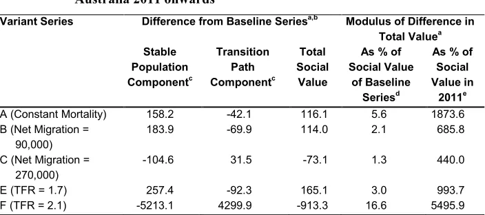
Table 5: Differences in components of social value and total social value in units between variant series and baseline series with diminishing returns to scale expressed on a per capita basis:
Australia 2011 onwards
Variant Series Difference from Baseline Seriesa,b Modulus of Difference in Total Valuea Stable
Population Componentc
Transition Path Componentc
Total Social
Value
As % of Social Value
of Baseline Seriesd
As % of Social Value in
2011e
A (Constant Mortality) 158.2 -42.1 116.1 5.6 1873.6 B (Net Migration =
90,000)
183.9 -69.9 114.0 2.1 685.8
C (Net Migration =
270,000) -104.6 31.5 -73.1 1.3 440.0 E (TFR = 1.7) 257.4 -92.3 165.1 3.0 993.7 F (TFR = 2.1) -5213.1 4299.9 -913.3 16.6 5495.9
Notes: a. Using gA= 1.5% p.a., ρ = 1.75% p.a., α= 0.95, and β = 0.
b. Expressed as a multiple of the 2011 the consumption value of one hour worked per week per capita. c. To facilitate comparison with Table 2 A0 has been scaled to equate Y/N = 16.6.
d. Value of baseline series = 5,511.0 times the consumption value of one hour worked per week per capita in 2011. e. As multiple of consumption value of 2011 Y/N (16.6).
size of the labour force to the further detriment of output per capita. However, when measured as a percentage of the value of 2011 output, the cost of projected mortality improvement is smaller under the diminishing returns to scale scenario than under constant returns (columns 5 in Tables 5 and 2), because under diminishing returns the influence of the more distant future, when the projected labour force size is larger, is reduced.
3.2.8 The effect of aversion to intergenerational inequality on social valuations
With a positive value for the parameter for aversion to intergenerational inequality (β) (Appendix A) the proportionate influence on the social valuation of projected values for
time points in the more distant future is reduced48, 49. Table 6 shows that, with the
higher discount rate resulting from the positive value of β, the direction of the effect of fertility on the consumption needs-weighted valuation is changed: the series TFR = 1.7 has a higher social value than the baseline series which, in turn, has a higher social
value than that of the high fertility series (TFR = 2.1)50. This reflects the reduced
proportionate influence on the valuations of the ‘post-crossover’ pattern of higher
values of Lt/Nt with higher fertility 47-51 years after the start of the projection, shown
by Figure 5. The sign of the effect of lower, as opposed to higher, fertility on the valuation depends on the estimated size of the parameter measuring aversion to intergenerational inequality (β), the consumption weights, the assumed trajectory for
labour force participation rates, and also on the choice of social discount rate (ρ)51. It
also depends on the specified assumptions for migration and mortality. For example, if a constant net migration of less than 92,000 per annum is assumed, as opposed to the baseline level of 180,000 per annum, a projection with total fertility of 1.7 will have a
48 This assumes the assumed rate of productivity growth, g
A, is positive.
49 Note the units of measurement for the components of the valuations in Table 5 are not comparable to those
for Tables 2 to 4.
50 The signs of the effects of these differences in fertility depend on the assumed trend for labour force
participation. Under the extrapolated trend for labour force participation the social value of the TFR = 1.7 series relative to the consumption needs-weighted population still exceeds that of the baseline (TFR=1.9) which, in turn, exceeds that for TFR=2.1. This reflects the higher rate of discount of the effects of future increases to labour force participation.
51For example, if the social discount rate (ρ) is less than 1.1%, the value of the TFR = 1.7 series is less than
lower (Cutler et al. 1990) consumption needs-weighted value than a series with the baseline level of total fertility (1.9)52.
Table 6: Differences in components of social value and total social value in units between variant series and baseline series for unweighted and consumption needs-weighted populations with incorporation of aversion to intergenerational inequality: Australia 2011 onwards Variant Series Difference from Baseline Seriesa,b Modulus of Difference in
Total Valuea Stable
Population Component
Transition Path Component
Total Social
Value Value of As % of Baseline Series
As % of Social Value
in 2011c
With N as (unweighted) Total Population
A (Constant Mortality) 1.04 -0.73 0.31 0.83 37.04 B (Net Migration =
90,000) 0.00 -0.17 -0.17 0.48 21.53 C (Net Migration =
270,000) 0.00 0.12 0.12 0.34 15.30 D (Net Migration = 0) -0.20 -0.28 -0.48 1.30 58.48 E (TFR = 1.7) 0.14 -0.01 0.14 0.37 16.75 F (TFR = 2.1) -0.07 -0.07 -0.14 0.40 17.83 With N Weighted for Relative Consumption Needsd
A (Constant Mortality) 1.38 -0.97 0.41 1.15 51.68 B (Net Migration =
90,000) 0.00 -0.26 -0.26 0.71 32.19 C (Net Migration =
270,000) 0.00 0.19 0.19 0.51 23.10 D (Net Migration = 0) -0.29 -0.41 -0.70 1.93 87.19
E (TFR = 1.7) 0.03 0.00 0.13 0.08 3.79
F (TFR = 2.1) -0.07 -0.11 -0.04 0.12 5.26
Notes: a. Using gA = 1.5% p.a., ρ = 1.75% p.a., and β = 1.4. b. Units of social utility per (unweighted or weighted) person.
c. 2011 L/N = 16.6 hours worked per week per unweighted person and 17.2 hours worked per week per consumption need-weighted person.
d. Using the weights of Cutler et al. (1990).
52This also assumes mortality follows the baseline series projected improvement, constant labour force