in the population sciences published by the Max Planck Institute for Demographic Research Konrad-Zuse Str. 1, D-18057 Rostock · GERMANY www.demographic-research.org
DEMOGRAPHIC RESEARCH
VOLUME 23, ARTICLE 8, PAGES 191-222
PUBLISHED 27 JULY 2010
http://www.demographic-research.org/Volumes/Vol23/8/ DOI: 10.4054/DemRes.2010.23.8
Research Article
Model migration schedules incorporating
student migration peaks
Tom Wilson
© 2010 Tom Wilson.
This open-access work is published under the terms of the Creative Commons Attribution NonCommercial License 2.0 Germany, which permits use, reproduction & distribution in any medium for non-commercial purposes, provided the original author(s) and source are given credit.
1 Introduction 192
2 The standard parameterized model migration schedule 195
3 The student peak parameterized model migration schedule 197
4 Fitting in Microsoft Excel 200
5 Illustrations 204
5.1 Example regions 204
5.2 Data 204
5.3 Student peak migration age schedules 205 5.4 The impact on population projections 206
6 Conclusions 216
7 Acknowledgements 217
Model migration schedules incorporating student migration peaks
Tom Wilson1
Abstract
This paper proposes an extension of the standard parameterized model migration schedule to account for highly age-concentrated student migration. Many age profiles of regional migration are characterized by sudden ‘spiked’ increases in migration intensities in the late teenage years, which are related to leaving school, and, in particular, to entry into higher education. The standard model schedule does not appear to be effective in describing the pattern at these ages. This paper therefore proposes an extension of the standard model through the addition of a student curve. The paper also describes a relatively simple Microsoft Excel-based fitting procedure. By way of illustration, both student peak and standard model schedules are fitted to the age patterns of internal migration for two Australian regions that experience substantial student migration. The student peak schedule is shown to provide an improved model of these migration age profiles. Illustrative population projections are presented to demonstrate the differences that result when model migration schedules with and without student peaks are used.
1 Queensland Centre for Population Research, School of Geography, Planning and Environmental
1. Introduction
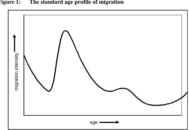
A fundamental characteristic of human migration patterns is the considerable similarity in regional migration age profiles across space and time. A large body of evidence has accumulated that demonstrates the extent of these regularities (see, for example, Rogers, Racquillet, and Castro 1978; Rees 1979; Rogers and Castro 1981; Bates and Bracken 1982; Rogers and Castro 1986; Rogers 1988; Rogers and Rajbhandary 1997; and Raymer and Rogers 2008). Figure 1 demonstrates the standard migration age profile. Migration intensities tend to peak in the young adult ages as individuals move to take up employment, educational, and partnering opportunities. They then decline with increasing age due to mobility-depressing influences, such as career stability, dual-career household formation, property ownership, and having children in school. Some migration age profiles contain a secondary peak in the fifties or sixties, as couples make housing adjustment moves, and/or shift to high amenity locations around retirement. Migration profiles that capture local moves may also show an increase at the oldest ages due to moves into institutions. The migration intensities of children echo those of their parents: moves are relatively frequent at the infant ages, when parents are younger and more mobile; then become less frequent until sometime in the teens; and then once again become more frequent as offspring begin to move out of the parental home.
Rogers, Racquillet, and Castro (1978) were the first to introduce a mathematical representation of the age pattern of migration, denoting it a model migration schedule. It has subsequently also been described as a parameterized model schedule and a multiexponential model schedule (because of the exponential functions in the equation). In the three decades since their introduction, model schedules have become firmly established as an important part of the toolbox of methods for the analysis of migration age patterns. Their uses include:
♦ estimation: where migration data are missing or suspect (e.g., Rogers and Jones 2008, Rogers, Jones and Ma 2008);
♦ graduation: especially where observed migration age patterns contain a lot of noise (e.g., Congdon 1993, Raymer and Rogers 2007);
♦ comparative analyses: a small number of parameters facilitates comparisons of migration age patterns over space and time (e.g., Rogers and Castro 1981, Ishikawa 2001);
♦ data reduction: a large number of age-specific migration intensities are replaced by a small number of parameters, thus reducing memory use in computer programmes for projections (e.g., Rees 1996); and
Figure 1: The standard age profile of migration
age
m
igr
at
ion
int
e
n
s
ity
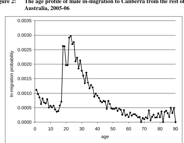
Much of the literature on model migration schedules has argued that they provide accurate descriptions of internal migration age patterns across the developed world and over time. While model schedules fit many contemporary migration age patterns quite well, there are some flows for which there are significant deviations from the standard model schedule, especially where single year of age and single year interval data are used. Higher education-related migration, which is highly concentrated in the late teenage years, is a case in point. For example, Figure 2 shows the age pattern of male in-migration to Canberra from the rest of Australia, as recorded by the 2006 Census. Canberra is home to several higher education institutions, and attracts a significant number of students from other regions of Australia. Clearly the standard model migration schedule as depicted in Figure 1 provides an unsatisfactory representation of this particular migration age pattern. How common are such migration age profiles in Australia? At the scale of Statistical Divisions,2 the majority of out-migration age profiles with single year of age detail clearly exhibit student peaks, whilst for in-migration age profiles, the peaks are most prominent in in-migration flows to metropolitan centers.
Figure 2: The age profile of male in-migration to Canberra from the rest of Australia, 2005-06
0.0000 0.0005 0.0010 0.0015 0.0020 0.0025 0.0030 0.0035
0 10 20 30 40 50 60 70 80 90
age
In
-m
igr
ati
on p
rob
abi
lity
Source: Calculated from Australian Bureau of Statistics 2006 Census data Note: In-migration probabilities are defined in section 5.2.
(e.g., ages 4-12 for primary school pupils in Queensland, and ages 13-17 for high school).
This paper proposes an extension of the standard model migration schedule, with the goal of achieving a better fit for age profiles which include a noticeable ‘spike’ in student migration. The proposed model schedule also replaces the original double exponential function used to represent the retirement curve with a three-parameter version that has more stable parameters. In addition, the paper describes a relatively simple Microsoft Excel-based fitting procedure, based on an awareness that some existing methods of fitting the model are quite technically demanding.
The plan of this paper is as follows. Following this introduction, the paper briefly presents the standard parameterized model migration schedule, as developed by Andrei Rogers and colleagues. In Section 3, the student peak version of the model schedule is presented. Section 4 describes the Microsoft Excel-based fitting procedure. Section 5 presents the student peak migration schedule using some Australian migration age patterns, as well as illustrative population projections that demonstrate the differences that result from using student peak schedules, rather than standard model schedules. The paper concludes with some suggestions for further research into model migration schedules.
2. The standard parameterized model migration schedule
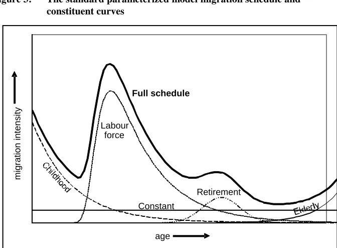
The standard model migration schedule is the sum of five component curves (Rogers and Watkins, 1987):
Migration intensity = childhood curve + labour force curve + retirement curve + elderly curve + constant.
Figure 3: The standard parameterized model migration schedule and constituent curves Constant Labour force Retirement Full schedule age m igr at io n i nt e n s it y
Source: based on Rogers and Watkins, 1987
Expressed algebraically, the full model migration schedule contains 13 parameters, and may be written as
(
)
(
)
(
)
{
}
(
)
(
)
{
}
(
)
1 12 2 2 2 2
3 3 3 3 3
4 4
ˆ ( ) exp
exp exp
exp exp
exp
m x a x
a x x
a x x
ˆ
m = modeled migration intensity, x = age,
1
a = height of the childhood curve,
1
α = rate of descent of the childhood curve,
2
α = height of the labour force curve,
2
λ = rate of ascent of the labour force curve,
2
α = rate of descent of the labour force curve,
2
µ = position of the labour force curve on the age axis,
3
a = height of the retirement curve,
3
λ = rate of ascent of the retirement curve,
3
α = rate of descent of the retirement curve,
3
µ = position of the retirement curve on the age axis,
4
a = height of the elderly curve,
4
α = rate of ascent of the elderly curve, and c = constant.
3. The student peak parameterized model migration schedule
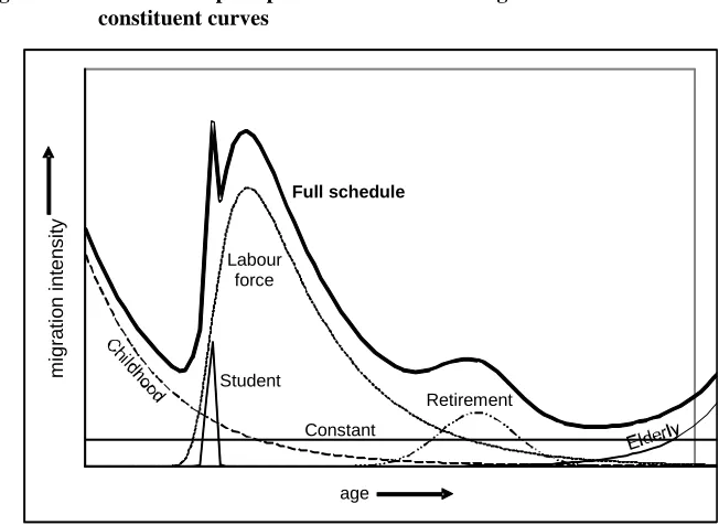
The student peak model migration schedule proposed here adds a student curve to represent highly age-focused student migration. The student peak model schedule is defined as
Migration intensity = childhood curve + labour force curve + retirement curve + elderly curve + student curve+ constant.
Figure 4: The student peak parameterized model migration schedule and constituent curves
Constant Student
Labour force
Retirement
Full schedule
age
m
ig
rat
ion
i
n
te
n
si
ty
The student curve is represented by the standard double exponential function
(
)
{
}
5 5 5 5 5 5
ˆ ( ) exp ( ) exp
m x =a −α x−µ − −λ x−µ (2)
where
5 ˆ
m = student component of the modelled migration intensity,
5
a = height of the student curve,
5
µ = position of the student curve on the age axis,
5
λ = rate of ascent of the student curve, and
5
α = rate of descent of the student curve.
A secondary refinement to the standard model is the replacement of the original double exponential retirement function. The replacement was made because attempts to fit this function resulted in considerable instability in the parameters. In its place, a three-parameter function employed by Peristera and Kostaki (2007) to represent the age profile of fertility was used. The Peristera-Kostaki function was chosen because of good fits to a number of test cases, the stability of its parameter estimates, and the intuitive meaning of the parameters: µ3 is the modal age of the distribution, a3 is the height of the curve, and σ3 determines whether the distribution is wide (large values) or narrow (small values). There is a small cost in using this model in that the function is symmetrical, but in most migration age patterns, this cost is unimportant. Thus
2 3
3 3
3
ˆ ( ) exp x
m x a µ
σ − = − (3) where 3 ˆ
m = retirement component of the modelled migration intensity,
3
a = height of the retirement curve,
3
µ = position of the retirement curve on the age axis, and
3
σ = rate of ascent and descent of the retirement curve.
It is interesting to note that, in his model migration schedule work for London, Congdon (1993) also replaced the double exponential of the retirement curve in order to obtain more easily interpretable parameters. He used a three-parameter function similar in form to the Peristera-Kostaki model.
The full student peak model schedule consists of 16 parameters, and is written as
(
)
(
)
(
)
{
}
(
)
(
)
(
)
{
}
1 12 2 2 2 2
2 3 3
3
4 4
5 5 5 5 5
ˆ ( ) exp
exp exp
exp
exp
exp exp
m x a x
a x x
x a
a x
a x x
where all parameters are as defined earlier. In some situations, more than one student curve may be present in a migration age pattern (for example, where there is also highly age-specific migration of boarding school pupils). When this is the case, another student curve can be added, and suitable subscripts can used to distinguish between them.
4. Fitting in Microsoft Excel
This section describes how the student peak model migration schedule may be fitted in a Microsoft Excel 2007 workbook, SPMMS.xlsm (available from the author on request). The workbook is designed to use single year interval, single year of age period -cohort migration data (Bell and Rees 2006) of the type typically obtained from a census or survey. Why is Excel used, rather than a statistical package with nonlinear regression routines? There are two reasons. First, one aim is to provide a method which can be used without difficulty for the purposes of graduation by individuals engaged in demographic research, but who lack access to, or knowledge of how to use, statistical software packages. Microsoft Excel is the most commonly used software for numerical work worldwide, and many professionals are highly experienced Excel users. Second, some of the existing programmes that have been used for fitting model migration schedules, such as MODEL (Rogers and Planck 1983) or Tablecurve2D (Rogers and Raymer 1999), require a considerable degree of expertise and experience to implement.
There are seven steps in the fitting procedure. Some aspects of this approach, including the disaggregation of m x( ) into separate components, are inspired by the linear estimation procedures described by Rogers, Castro, and Lea (2005).
Step 1: Place input data into the Excel workbook
Step 2: Estimate the constant
The value of the constant is estimated as the mean of between one and 15 of the lowest non-zero scaled migration intensities (with a default of five). In the SPMMS.xlsm workbook, a graph showing the scaled probabilities and the constant is provided to guide the user on how many of the lowest intensities to include.
Step 3: Estimate the childhood curve parameters
The childhood curve parameters are fitted to the scaled migration intensities, minus the constant
( )
( )
1
m x =m x −c. (5)
Modelled values of m x1( ), represented by the function
( )
(
)
1 1 1
ˆ exp
m x =a −α x , (6)
are estimated by creating the linear model
Y= +C M X (7)
where
( )
(
)
( )
11
1 ln
ln
Y m x
C a
M α
= = = − X =x.
The Excel functions SLOPE and INTERCEPT provide the values of C and M, thus giving
( )
1 expa = C
1 M
Guided by a graph showing m x1( ) and the fitted childhood curve in the SPMMS.xlsm workbook, the user can alter the default ages over which the childhood curve is fitted (one to 14) if doing so appears to give a better fit.
Step 4: Estimate the labour force curve parameters
The labour force curve parameters are fitted to the scaled migration intensity, minus the constant and the childhood curve
( )
( )
( )
2 ˆ1
m x =m x − −c m x . (8)
The function
( )
{
(
)
(
)
}
2 2 2 2 2 2
ˆ exp exp
m x =a −α x−µ − −λ x−µ (9)
is fitted using Microsoft Excel’s nonlinear regression facility, Solver. Over a user-defined age range (with a default of 17 to 49, usually excluding 18, 19, and 20 for the student curve) the function is fitted to minimize the sum of squared residuals. Attempts to use Solver on a variety of migration age patterns resulted in good fits being obtained almost every time. The use of Solver here raises the question of why it is not used to fit the full model schedule in one step. Solver works well when handling up to four or five parameters. However, its iterative search algorithm tends to fail to converge, or produces a nonsensical result, when a larger number of parameters are introduced.
Step 5: Estimate the retirement curve parameters
A checkbox in the SPMMS.xlsm workbook is used to determine whether the retirement curve is included in the model schedule. If the checkbox is ticked, then the retirement curve parameters are fitted over a user-defined age range to the scaled migration intensities, minus the constant, childhood curve, and labour force curve, m x3( ), where
( )
( )
( )
( )
3 ˆ1 ˆ2
m x =m x − −c m x −m x . (10)
( )
3 23 3
3
ˆ exp x
m x a µ
σ −
= −
. (11)
Step 6: Estimate the elderly curve parameters
A checkbox must also be ticked to include the elderly curve in the model schedule. If this function is needed, then it is fitted over a user-defined age range to the values of
4( )
m x , defined as
( )
( )
( )
( )
( )
4 ˆ1 ˆ2 ˆ3
m x =m x − −c m x −m x −m x . (12)
Excel Solver is used to estimate the parameters of the function:
( )
(
)
4 4 4
ˆ exp
m x =a α x . (13)
The linearization method used for the childhood curve is not used in this case because some values of m x4( ) are likely to be negative, and logarithms therefore cannot be calculated.
Step 7: Estimate the student curve parameters
To add the student curve to the model schedule, a checkbox must be ticked in the workbook. A graph showing the fitted model schedule so far and m x5( ), where
( )
( )
( )
( )
( )
( )
5 ˆ1 ˆ2 ˆ3 ˆ4
m x =m x − −c m x −m x −m x −m x , (14)
guides the user on the ages over which the student curve is best fitted. Excel Solver is then employed to find the parameters of the function
( )
{
(
)
(
)
}
5 5 5 5 5 5
ˆ exp exp
5. Illustrations
5.1 Example regions
In Australia, the spatial pattern of higher education-related internal migration consists primarily of rural and smaller city residents moving to a metropolitan area to access a wide range of courses and attend the more prestigious universities, whilst the age pattern is characterized by considerable concentration over the late teenage years to the early twenties (Blakers et al. 2003, Mills 2006). To illustrate the student peak model migration schedule, two regions with migration age patterns that are typical of metropolitan and non-metropolitan regions were chosen: the Statistical Divisions of Brisbane and Mackay. Brisbane, the state capital of Queensland, is home to about two million people, and is a major higher education centre serving much of Queensland, as well as northern New South Wales. Mackay is a region of central Queensland located just north of the Tropic of Capricorn. It has a population of about 170,000, and offers limited higher education opportunities.
5.2 Data
Migration data by sex and single years of age were obtained from the Australian Bureau of Statistics 2006 Census (via its TableBuilder service [ABS 2009]). These data were derived from the following census questions: “Where does the person usually live?” and “Where did the person usually live one year ago (on 8 August 2005)?” (ABS 2006). These are therefore transition-type data, and count surviving migrants rather than migrations (Courgeau 1979, Rees and Willekens 1985). The migration intensity used in this study was the intensity recommended for this type of data by Rees et al. (2000), or the migration probability conditional upon survival within the country (hereafter, just migration probability). For out-migration from any particular region, the migration probability for each cohort was calculated as:
Out-migration probability =
People resident in the region one year before the census who were living elsewhere in Australia on census night
For in-migration, the migration probability for each cohort was calculated as:
In-migration probability =
People resident anywhere in Australia except the region one year before the census who were living in the region on census night
People resident anywhere in Australia except the region one year before the census who were living anywhere in Australia on census night
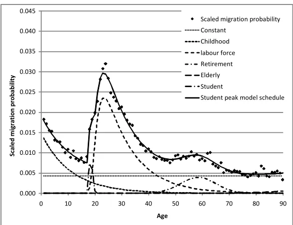
5.3 Student peak migration age schedules
Figures 5 to 8 illustrate student peak model migration schedules fitted to the female in- and out-migration age patterns of Brisbane and Mackay using the SPMMS.xlsm workbook. As male and female age patterns are very similar, only the female age patterns are shown to avoid repetition. Age in the graphs refers to the mean exact age of each cohort in the one-year interval (for example, the cohort aged 17 at their last birthday one year prior to the census, and aged 18 on their last birthday on the census night, have a mean age at migration of 18.0 years in the one year interval).
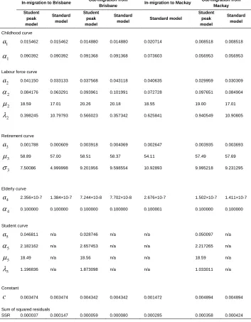
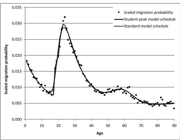
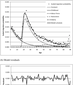
Part (a) of Figures 5, 6, and 8 shows the student peak model schedules and constituent curves (for in-migration to Mackay, shown in Figure 7, there was no need for a student curve, so a standard model schedule was fitted). Part (b) compares the student peak model schedule against the standard model without the student curve (except for Figure 7). The standard model schedule was fitted using the SPMMS.xlsm workbook except that the student curve was excluded. Note that the three-parameter Peristera-Kostaki function was also used for the retirement curve in the ‘standard’ model. Part (c) of each figure (apart from Figure 7) displays the residuals for both type of model schedule, where the model residuals are defined as the model schedule value,
ˆ ( )
m x , minus the scaled migration probability, m x( ). Table 1 lists the parameters and sum of squared residuals for each model schedule.
student peak schedule. For the out-migration from Mackay, the improvement is from 0.000424 to 0.000358.
5.4 The impact on population projections
Achieving good model fits is particularly important for population projections which make use of migration intensities graduated with model migration schedules. If incorrect numbers of migrants are being projected into and out of a region’s population at specific ages, inaccurate population projections will result for those ages, and then propagate to older ages as the affected cohorts age over time. Incorrectly projected age groups will in turn affect subsequent projections of migration, fertility, and mortality.
But just how much difference does the student peak migration schedule make in a projection application? Is the difference significant enough to warrant the use of the student peak model? The answer will, of course, depend on the extent to which there is highly age-specific student migration in the system being modeled. To provide a simple illustration, two sets of population projections for Brisbane were prepared with a cohort-component bi-regional model (Rogers 1976) for the period 2006-26. The first set employed standard model migration schedules, whilst the second set applied the student peak migration schedules. All input data and assumptions were identical except for the internal migration age schedules.
Table 1: Model schedule parameters and sum of squared residuals
In-migration to Brisbane Out-migration from
Brisbane In-migration to Mackay
Out-migration from Mackay Student peak model Standard model Student peak model Standard
model Standard model
Student peak model Standard model Childhood curve 1
a 0.015462 0.015462 0.014880 0.014880 0.020714 0.008518 0.008518
1
α 0.090392 0.090392 0.091368 0.091368 0.073603 0.056953 0.056953
Labour force curve
2
a 0.041150 0.033133 0.037568 0.043118 0.040635 0.029959 0.030309
2
α 0.084176 0.063291 0.093961 0.101991 0.072728 0.097651 0.084904
2
µ 18.59 17.01 20.26 20.18 18.55 19.00 17.01
2
λ 0.398245 10.79793 0.566023 0.357342 0.625841 0.940549 10.90805
Retirement curve
3
a 0.001788 0.000609 0.003918 0.004069 0.002647 0.003935 0.003693
3
µ 58.89 57.00 58.51 58.37 54.11 57.49 57.69
3
σ 7.50086 4.999998 9.201956 9.598554 10.92893 9.995218 9.231295
Elderly curve
4
a 2.356×10⁻⁷ 1.384×10⁻⁷ 7.244×10⁻⁸ 7.702×10⁻⁸ 2.676×10⁻⁷ 1.502×10⁻⁷ 1.411×10⁻⁷
4
α 0.100000 0.100000 0.100000 0.100000 0.100001 0.100000 0.100000
Student curve
5
a 0.046811 n/a 0.028746 n/a n/a 0.050097 n/a
5
α 2.182162 n/a 2.657453 n/a n/a 2.217265 n/a
5
µ 18.49 n/a 18.56 n/a n/a 18.59 n/a
5
λ 1.196836 n/a 1.873098 n/a n/a 1.033011 n/a
Constant
c 0.003474 0.003474 0.004342 0.004342 0.001472 0.004894 0.004894 Sum of squared residuals
Figure 5: Female in-migration to Brisbane statistical division, 2005-06
(a) Full student peak model schedule and constituent functions
0.000 0.005 0.010 0.015 0.020 0.025 0.030 0.035 0.040 0.045
0 10 20 30 40 50 60 70 80 90
Age
Scaled migration probability Constant
Childhood labour force Retirement Elderly Student
Student peak model schedule
Sc
al
ed
m
ig
ra
tion
p
rob
ab
ili
Figure 5: (Continued)
(b) Comparison of student peak and standard model migration schedules
0.000 0.005 0.010 0.015 0.020 0.025 0.030 0.035 0.040 0.045
0 10 20 30 40 50 60 70 80 90
Sc le d m ig ra tio n p ro ba bilit y Age
Scaled migration probability Student peak model schedule Standard model schedule
0.000 0.005 0.010 0.015 0.020 0.025 0.030 0.035 0.040 0.045
0 10 20 30 40 50 60 70 80 90
Age
Scaled migration probability Student peak model schedule Standard model schedule
Sc al ed m ig ra tion p rob ab ili ty
(c) Comparison of student peak and standard model residuals
-0.010 -0.005 0.000 0.005 0.010
0 10 20 30 40 50 60 70 80 90
Re
sid
ua
ls
Age
Student peak model residuals Standard model residuals
-0.010 -0.005 0.000 0.005 0.010
0 10 20 30 40 50 60 70 80 90
Age
Student peak model residuals Standard model residuals
Re
si
du
Figure 6: Female out-migration from Brisbane statistical division, 2005-06
(a) Full student peak model schedule and constituent functions
0.000 0.005 0.010 0.015 0.020 0.025 0.030 0.035 0.040 0.045
0 10 20 30 40 50 60 70 80 90
Age
Scaled migration probability Constant
Childhood labour force Retirement Elderly Student
Student peak model schedule
Sc
al
ed
m
ig
ra
tion
p
rob
ab
ili
Figure 6: (Continued)
(b) Comparison of student peak and standard model migration schedules
0.000 0.005 0.010 0.015 0.020 0.025 0.030 0.035
0 10 20 30 40 50 60 70 80 90
Age
Scaled migration probability Student peak model schedule Standard model schedule
Sc
al
ed
m
ig
ra
tion
p
rob
ab
ili
ty
(c) Comparison of student peak and standard model residuals
-0.010 -0.005 0.000 0.005 0.010
0 10 20 30 40 50 60 70 80 90
Age
Student peak model residuals Standard model residuals
Re
si
du
Figure 7: Female in-migration to Mackay statistical division, 2005-06
(a) Full model schedule and constituent functions
0.000 0.005 0.010 0.015 0.020 0.025 0.030 0.035 0.040 0.045
0 10 20 30 40 50 60 70 80 90
Age
Scaled migration probability Constant
Childhood labour force Retirement Elderly Model schedule
Sc
al
ed
m
ig
ra
tion
p
rob
ab
ili
ty
(b) Model residuals
-0.010 -0.005 0.000 0.005 0.010
0 10 20 30 40 50 60 70 80 90
Age
Re
si
du
Figure 8: Female out-migration from Mackay statistical division, 2005-06
(a) Full student peak model schedule and constituent functions
0.000 0.005 0.010 0.015 0.020 0.025 0.030 0.035 0.040 0.045
0 10 20 30 40 50 60 70 80 90
Age
Scaled migration probability Constant
Childhood labour force Retirement Elderly Student
Student peak model schedule
Sc
al
ed
m
ig
ra
tion
p
rob
ab
ili
Figure 8: (Continued)
(b) Comparison of student peak and standard model migration schedules
0.000 0.005 0.010 0.015 0.020 0.025 0.030 0.035 0.040 0.045
0 10 20 30 40 50 60 70 80 90
Age
Scaled migration probability Student peak model schedule Standard model schedule
Sc al ed m ig ra tion p rob ab ili ty
(c) Comparison of student peak and standard model residuals
-0.010 -0.005 0.000 0.005 0.010
0 10 20 30 40 50 60 70 80 90
Re
sid
ua
l
Age
Student peak model residuals Standard model residuals
-0.010 -0.005 0.000 0.005 0.010
0 10 20 30 40 50 60 70 80 90
Age
Student peak model residuals Standard model residuals
Re
si
du
Figure 9: Comparison of projected female net internal migration using the standard and student peak model migration schedules, Brisbane, 2015-16
(a) Net internal migration projections
-200 0 200 400 600 800 1000 1200 1400
0 10 20 30 40 50 60 70 80 90
Age in 2016
Student peak model Standard model
N
et
in
te
rn
al
m
ig
ra
tio
n 2
01
5-16
(b) Difference in net internal migration projections (student peak minus standard)
-200 -100 0 100 200
0 10 20 30 40 50 60 70 80 90
Age in 2016
N
et i
nter
na
l m
ig
ra
tio
n d
iff
er
en
Figure 10: Comparison of projected female population age structures using the standard and student peak model migration schedules, Brisbane, 2016 and 2026
0,000 5,000 10,000 15,000 20,000 25,000
0 10 20 30 40 50 60 70
Age
Student peak model Standard model
2026
2016
2006 (jump-off)
Po
pu
lat
io
n
6. Conclusions
Some further avenues for research on model migration schedules present themselves. First, in what ways do these “spiked” student migration age profiles vary across space, both within countries and internationally, and at what spatial scales are they most apparent? Second, how has the student component of migration age profiles evolved over time, and how might it evolve in the future? One possibility is that it will become more prominent in age patterns as the age at which individuals begin tertiary education remains the same, but that the labour force curve will continue to age slowly. Third, the student peak model schedule proposed here used the standard double exponential function. Some experimentation with other functions may prove worthwhile, especially if the number of parameters can be reduced. Fourth, how do the fits obtained from the SPMMS.xlsm workbook compare with those available through other statistical packages, such as Tablecurve2D and R? Fifth, what forms do migration age profiles take at the very highest ages? Although migrant numbers are small at these ages, the elderly represent a rapidly growing segment of developed countries’ populations. Aggregating migration flows between types of areas should enable some patterns to emerge. Sixth, international migration age profiles have received little attention in model migration schedule work. In the context of significant international student migration, what sort of model schedules are most appropriate for representing immigration and emigration?
7. Acknowledgements
I am grateful to Professor Martin Bell, Dr. James Raymer and two anonymous referees for their helpful comments on an earlier draft of this paper. All errors and shortcomings, of course, remain my own.
Corrections:
References
ABS (Australian Bureau of Statistics) (2006). How Australia Takes a Census. ABS Catalogue Number 2903.0. Canberra: ABS: 68 pp.
ABS (Australian Bureau of Statistics) (2009). TableBuilder [electronic resource: Australian 2006 Census web-based data extraction service] Canberra: ABS.
www.abs.gov.au/TableBuilder.
Bates, J. and Bracken, I. (1982) Estimation of migration profiles in England and Wales. Environment and Planning A 14(7): 889-900. doi:10.1068/a140889.
Bell, M. (1995). Internal Migration in Australia 1986-1991: Overview Report. Canberra: Australian Government Publishing Service.
Bell, M. and Rees, P. (2006). Comparing migration in Britain and Australia: harmonisation through use of age-time plans. Environment and Planning A 38(5): 959-988. doi:10.1068/a35245.
Blakers, R., Bill, A., Maclachlan, M. and Karmel, T. (2003) Mobility: Why Do University Students Move? Canberra: Department of Education, Science and Training: 35 pp.
Congdon, P. (1993). Statistical graduation in local demographic analysis and projections. Journal of the Royal Statistical Society Series A 156(2): 237-270.
doi:10.2307/2982731.
Courgeau, D. (1979). Migrants and migrations. Population: Selected Papers 3: 1-35. Freeman, R.B. (2009). What does global expansion of higher education mean for the
US? Cambridge, MA: National Bureau of Economic Research. (NBER Working Paper 14962). [Accessed from http://www.nber.org/papers/w14962 on 9th November 2009]
Ishikawa, Y. (2001). Migration turnarounds and schedule changes in Japan, Sweden and Canada. Review of Urban and Regional Development Studies 13(1): 20-33. Mills, J. (2006). Student Residential Mobility in Australia – An Exploration of Higher
Education-Related Migration. [Honours thesis]. Brisbane: The University of Queensland, School of Geography, Planning and Architecture.
Plane, D.A. and Heins, F. (2003). Age articulation of US inter-metropolitan migration flows. The Annals of Regional Science 37(1): 107-130.
Raymer, J. and Rogers, A. (2007). The American Community Survey’s interstate migration data: strategies for smoothing irregular age patterns. Southampton: Southampton Statistical Sciences Research Institute: 16pp. (Southampton Statistical Sciences Research Institute Methodology Working Paper M07/13). [Accessed from http://eprints.soton.ac.uk/48352/ on 3rd February 2008]
Raymer, J. and Rogers, A. (2008). Applying model migration schedules to represent age-specific migration flows. In: Raymer, J. and Willekens, F. (eds.). International Migration in Europe: Data, Models and Estimates. Chichester: Wiley: 175-192.
Rees, P. (1996). Projecting the national and regional populations of the European Union using migration information. In: Rees, P., Convey, A., and Kupiszewski, M. (eds.). Population Migration in the European Union. Chichester: John Wiley: 331-364.
Rees, P. and Willekens, F. (1985). Data and accounts. In: Rogers, A. and Willekens, F. J. (eds.). Migration and Settlement: A Multiregional Comparative Study. Dordrecht: D Reidel: 19-58.
Rees, P.H. (1979). Migration and Settlement: 1. United Kingdom. Research Report RR-79-3. Laxenburg: International Institute for Applied Systems Analysis.
Rees, P., Bell, M., Duke-Williams, O., and Blake, M. (2000). Problems and solutions in the measurement of migration intensities: Britain and Australia compared. Population Studies 54(2): 207-222. doi:10.1080/713779082.
Rogers, A. (1976). Shrinking large-scale population projection models by aggregation and decomposition. Environment and Planning A 8(5): 515-541. doi:10.1068/ a080515.
Rogers, A. (1986). Parameterized multistate population dynamics and projections. Journal of the American Statistical Association 81(393): 48-61. doi:10.2307/ 2287967.
Rogers, A. (1988). Age patterns of elderly migration: an international comparison. Demography 25(3): 355-370. doi:10.2307/2061537.
Rogers, A. and Castro, L.J. (1986). Migration. In: Rogers, A. and Willekens, F.J. (eds.). Migration and Settlement: A Multiregional Comparative Study. Dordrecht: D Reidel: 157-208.
Rogers, A. and Jones, B. (2008). Inferring directional migration propensities from the propensities of infants in the United States. Mathematical Population Studies 15(3):182-211. doi:10.1080/08898480802222283.
Rogers, A. and Planck, F. (1983). MODEL: A general program for estimating parameterized model schedules of fertility, mortality, migration and marital and labor force status transitions. Laxenburg: International Institute for Applied Systems Analysis. (Working Paper WP-83-102).
Rogers, A. and Raymer, J. (1999). Fitting observed demographic rates with the multiexponential model schedule: an assessment of two estimation programs. Review of Urban and Regional Development Studies 11(1): 1-10.
doi:10.1111/1467-940X.00001.
Rogers, A. and Watkins, J. (1987). General versus elderly interstate migration and population redistribution in the United States. Research on Aging 9(4): 483-529.
doi:10.1177/0164027587094002.
Rogers, A. and Rajbhandary, S. (1997). Period and cohort age patterns of US migration, 1948-1993: Are American males migrating less? Population Research and Policy Review 16(6): 513-530. doi:10.1023/A:1005824219973.
Rogers, A., Castro, L.J., and Lea, M. (2005). Model migration schedules: three alternative linear estimation methods. Mathematical Population Studies 12(1): 17-38. doi:10.1080/08898480590902145.
Rogers, A., Jones, B., and Ma, W. (2008). Repairing the migration data reported by the American Community Survey. Boulder: University of Colorado at Boulder, Institute of Behavioral Science. (Working Paper, Population Program).
Rogers, A., Racquillet, R. and Castro, L.J. (1978). Model migration schedules and their applications. Environment and Planning A 10(5): 475-502.
doi:10.1068/a100475.
Schofer, E. and Meyer, J.W. (2005). The worldwide expansion of higher education in the twentieth century. American Sociological Review 70(6): 898-920.