Determination of Mueller matrix elements in the presence of imperfections in optical components

University of New Orleans University of New Orleans

ScholarWorks@UNO

ScholarWorks@UNO

University of New Orleans Theses and

Dissertations Dissertations and Theses

5-15-2009

Determination of Mueller matrix elements in the presence of

Determination of Mueller matrix elements in the presence of

imperfections in optical components

imperfections in optical components

University of New Orleans

Follow this and additional works at: https://scholarworks.uno.edu/td

Recommended Citation Recommended Citation

Chakraborty, Shibalik, "Determination of Mueller matrix elements in the presence of imperfections in optical components" (2009). University of New Orleans Theses and Dissertations. 969.

https://scholarworks.uno.edu/td/969

This Thesis is protected by copyright and/or related rights. It has been brought to you by ScholarWorks@UNO with permission from the rights-holder(s). You are free to use this Thesis in any way that is permitted by the copyright and related rights legislation that applies to your use. For other uses you need to obtain permission from the rights-holder(s) directly, unless additional rights are indicated by a Creative Commons license in the record and/or on the work itself.

Determination of Mueller matrix elements in the presence of imperfections in

optical components

A Thesis

Submitted to the Graduate Faculty of the University of New Orleans

In partial fulfillment of the requirements for the degree

Master of Science In

Electrical Engineering

by

Shibalik Chakraborty

B.Tech, West Bengal University of Technology, Calcutta, India, 2007

ii

ACKNOWLEDGEMENT

First of all I would like to thank my graduate supervisor, Professor Rasheed Azzam, who

helped and encouraged me to start my graduate studies at the University of New Orleans in the

Electrical Engineering Department. I also thank him for his guidance, patient support, and for

proposing to me a very interesting research subject. I would like to thank Dr. Vesselin Jilkov and

Dr. Huimin Chen for serving as members of my thesis committee. Finally, I wish to dedicate this

iii

TABLE OF CONTENTS

List of Tables………...v

List of Figures……….vi

Abstract………...vii

Chapter 1. Introduction………..1

Chapter 2. Optical System and Modification………9

2.1. Introduction……….9

2.2. Fourieranalysis with ideal conditions……….13

2.3. Mueller matrix ……….………..13

Chapter 3. Offsets and Imperfections……….………..14

3.1. Introduction………..14

3.2. Fourier analysis and determination of offsets and imperfection parameters from Fourier coefficients……….15

Chapter 4. Determination of Mueller matrix elements……….26

4.1. Introduction………26

iv

4.3. Determination of Mueller-matrix elements……….………29

5. Summary………..32

6. Future Work……….………..33

References……….………34

v

LIST OF TABLES

Table 2.1: Fourier coefficients of the detected signal for the modified optical arrangement in

ideal conditions

Table 3.1: Fourier coefficients for the straight-through configuration with an offset azimuth for

the fixed analyzer

Table 3.2: Fourier coefficients for the straight-through configuration when the phase angles (α

and β) of the rotating components are introduced

Table 3.3: Fourier coefficients for the configuration without rotating analyzer

Table 3.4: Fourier coefficients in terms of the azimuth of fixed analyzer (A’) and its imperfection

parameters (ρ and δ)

Table 4.1: Interrelationship between the Mueller matrix elements mij (i,j=0,..,3) and the Fourier

vi

LIST OF FIGURES

Fig. 1.1: Four parameters that define the ellipse of polarization in its plane

Fig. 1.2: Polarizer orientation and azimuth

Fig. 1.3: System of n optical devices

Fig. 2.1: The original Polarizer-Sample-Analyzer (PSA) arrangement

Fig. 2.2: The modified arrangement by adding the fixed polarizer and analyzer at the ends

Fig. 3.1: Straight-through configuration with the polarizer and analyzer in line

Fig. 3.2: Straight-through configuration without the rotating analyzer

Fig. 3.3: Straight-through configuration with all the parameters

Fig. 4.1: Measurement configuration with the sample reintroduced between the rotating

vii

ABSTRACT

The Polarizer-Sample-Analyzer (PSA) arrangement with the optical components P and A

rotating with a fixed speed ratio (3:1) was originally introduced to determine nine Mueller

matrix elements from Fourier analysis of the output signal of a photodetector. The

arrangement is modified to the P’PSAA’ arrangement where P’ and A’ represent fixed polarizers

that are added at both ends with the speed ratio of the rotating components (P and A)

remaining the same as before. After determination of the partial Mueller matrix in the ideal

case, azimuthal offsets and imperfection parameters are introduced in the straight-through

configuration and the imperfection parameters are determined from the Fourier coefficients.

Finally, the sample is reintroduced and the full Mueller matrix elements are calculated to show

the deviation from the ideal case and their dependency on the offsets and imperfection

parameters.

8

CHAPTER 1

INTRODUCTION

Polarization is a property that is common to all vector waves. It is defined by the

behavior with time of one of the field vectors appropriate to that wave, observed at a fixed

point in space. Light waves are electromagnetic in nature and are described by four field

vectors: electric field strength E , electric displacement density D , magnetic field strength H , and

magnetic flux density B . The electric field strength E is used to define the state of polarization.

This is because the force exerted on electrons by the electric field is much greater than that

exerted by the magnetic field of the wave. The polarization of the three field vectors can be

determined using the Maxwell’s field equations, once the polarization of E has been

determined [1].

Ellipsometry is an optical technique for the characterization of interfaces and films and

is based on the polarization transformation that occurs as a beam of polarized light is reflected

from or transmitted through the interfaces or films [1].

We now present the four parameters that define an ellipse of polarization and we will

9

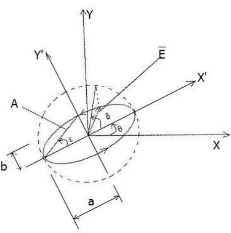
Fig 1.1. Four parameters defining the ellipse of polarization in its plane (1) the azimuth θ of the major axis from a fixed direction X, (2) the ellipticity e=±b/a=±tan ε, (3) the amplitude A=(a2+ b2)1/2 and (4) the absolute phase δ.

(1) The azimuth θ is the angle between the major axis the ellipse and the positive direction of

the X axis and defines the orientation of the ellipse.

- π₂≤ θ < π₂ (1.1)

(2) The ellipticity e is the ratio of the semi-minor axis of the ellipse b to the semi-major axis a,

e= b

a

10

A= a2+ b2 1/2 (1.3)

(4) The absolute phase vector δ determines the angle between the initial position of the electric

vector at t=0 and the major axis of the ellipse. All possible values of δ are limited by

-π ≤ δ < π (1.4)

The electric vectors of light linearly polarized in the X and Y directions are given by,

E x= Axcos(ωt+φx)i (1.5)

E y= Aycos(ωt+φy)j (1.6)

For elliptically polarized light the electric vector is then given by

E = E x+E y= Axcos(ωt+φx)i + Aycos(ωt+φy)j (1.7)

Or in matrix (column) form as,

E = E x

E _y =

Axei(ωt+φx) A_yej(ωt+φy) = e

jωt_{𝐉 (1.8)}

Taking out the time dependence from Eq. (1.8), we have the Jones vector

𝐉= Axe iφx

A_yeiφy (1.9)

11

E′_x E′_y =

t₁₁ t₁₂ t₂₁ t₂₂

E_x

Ey (1.10)

or

𝐉’=𝐓𝐉 (1.11)

Here 𝐓 is defined as the Jones matrix of the optical system, the matrix elements t ij are

determined from the known properties of the optical element encountered by the light and the

equation is simply the transformation matrix that converts 𝐉 into 𝐉’.

Similar to the Jones calculus, the Mueller calculus also represents the light by a vector;

premultiplication of this vector by a matrix that represents an optical element yields a resultant

vector that describes the beam after its interaction with the optical device. The vector

representing the light is called a Stokes vector and is a 4 X 1 real vector instead of 2 X 1 complex

Jones vector. The 4 elements of the Stokes vector represent intensities of the light. Therefore

these elements are real. A common representation of the Stokes vector is given by

𝐒= S₀ S₁ S2 S₃ =

Ax2+ Ay2 Ax2− Ay2 2AxAycosδ 2A_xA_ysinδ

(1.12)

where δ =δy- δx and –π≤ δ ≤π.

A deterministic complex Jones matrix cannot be used to express the depolarizing incoherent

12

powerful Mueller matrix. The output coherency vector can be written in terms of the input

coherency vector as

𝐉₀ = (T x 𝐓∗)𝐉i (1.13)

The coherency vector J can be related to the Stokes vector S as S = AJ,1

where A =

1 0

1 0 00 −11

0 1

0 −j 1 0j 0

(1.14)

The relationship between the Stokes vector 𝐒o and 𝐒i of the outgoing and incident waves is

given by,

𝐒₀ = [A(T x 𝐓∗)𝐀−𝟏]𝐒i or 𝐒0 = M𝐒i (1.15)

where M = A(T x 𝐓∗)𝐀−𝟏

We now introduce the main optical device that is used in the optical measurement

13

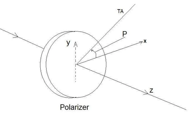
Fig 1.2. The polarizer azimuth P is measured from the positive X direction as a reference in an anticlockwise sense. The direction Z is the direction of propagation of light. TA is the transmission axis of the polarizer.

A linear polarizer transmits a beam of light whose electric field vector oscillates in a

plane that contains the beam axis and transmission axis TA. The orientation of this plane in

space can be varied by rotation of the polarizer about the beam axis. As shown Fig 1.2, the

azimuth of the polarizer P is measured from the positive direction of X axis, where Z is the

direction of propagation of light.

The Jones matrix of any optical device is a function of the azimuthal orientation of the

14

The matrix 𝐓’ for a linear polarizer or retarder with its optical axis rotated by an angle θ from

the coordinates is found from T by a matrix rotation such that

𝐓’=R(-θ)TR(θ) (1.16)

where R(θ) = cosθ_{−sinθ cosθ}sinθ (1.17)

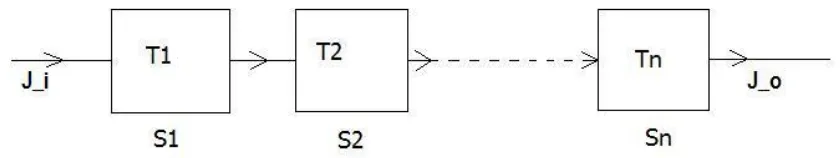
For a system of devices as shown below the resulting Jones vector is given by

Fig 1.3. A combined effect of n optical systems S1, S2,…,Sn of Jones Matrix T1, T2,…, Tn.

𝐉’ = Tn𝐉’’ (1.18)

𝐉’’ = Tn−1𝐉’’’ (1.19)

So the combination of the system of devices will give

15

where Ti is the Jones matrix for the ith element and 𝐉i is the Jones vector at the input. A similar

analysis applies in the Stokes Mueller matrix calculus as will be used in subsequent chapters.

16

CHAPTER 2

OPTICAL SYSTEM AND MODIFICATION

2.1 Introduction

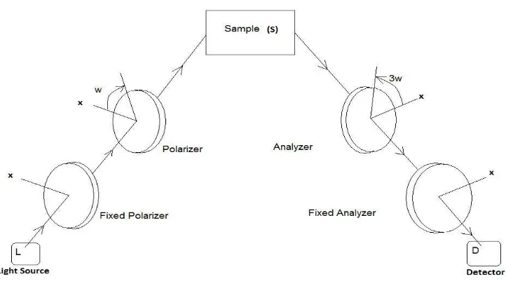
The original arrangement [2] is that of a typical ellipsometric arrangement with the

sample placed between a polarizer and analyzer. The polarizer and analyzer are rotated with a

fixed speed ratio of 3:1 respectively. The figure below shows this arrangement and the

directions of rotation and azimuths of the optical elements. The 3:1 speed ratio is important in

the fact that it gives the best results in terms of linearity of the obtained Mueller matrix

elements in terms of the Fourier coefficients.

17

Nine elements of the sample Mueller matrix for the above arrangement are obtained as linear

combination of the Fourier coefficients of the detected signal. The light source L is unpolarized,

circularly polarized or partially circularly polarized. A depolarizer is needed in front of the

detector to have a polarization insensitive photodetector as the polarization of light leaving the

analyzer varies with time.

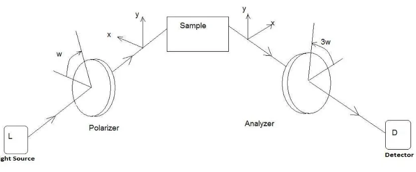
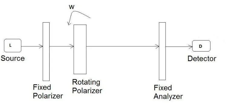
The photopolarimeter arrangement of Fig. 2.1 is modified by adding a fixed polarizer

(FP) and fixed analyzer (FA) at the beginning and end as shown in Fig. 2.2. The direction x and y

are parallel and perpendicular, respectively, to the scattering plane described by the directions

of incident and transmitted light.

Fig 2.2. Fourier photopolarimeter with added fixed polarizer and analyzer. S is the optical system under measurement; L and D are the light source and detector respectively. x and y are parallel and perpendicular to the

18

2.2 Fourier analysis with ideal conditions

The azimuths of the rotating polarizer and analyzer P and A are measured from the

positive direction of the x axis. Let 𝐒FP be the Stokes vector of light leaving the polarizer, ГFA

the first row of the Mueller matrix of the fixed analyzer, 𝐌A the Mueller matrix of the rotating

analyzer, 𝐌P the Mueller matrix of the rotating polarizer and 𝐌S the Mueller matrix of the

sample under measurement. Then the output signal of the detector D is given by the equation,

i= kГFA𝐌A𝐌S𝐌P𝐒FP, (2.1)

where k represents the detector sensitivity. Now substituting 𝐒FP = I[1 cos(2P′) sin(2P′) 0]T

(where I is the intensity of light leaving thepolarizer and T indicates transpose), 𝐌S= (mij), i,

j=1,2,3,4 , ГFA = τ*1 cos2A’ sin2A’ 0+, 𝐌Aand 𝐌P are the Mueller matrices of the rotating

analyzer and polarizer. Taking the fixed polarizer to have zero azimuth, we have the Stokes

vector 𝐒FP = [1 1 0 0]T. Putting all these values in Eqn. (2.1), we get

i= XY[ m11 + m12cos(2P) + m13sin(2P) + m21cos(2A) + m22cos(2A)cos(2P) + m23sin(2P)cos(2A) +

m₃₁sin(2A) + m32sin(2A)cos(2P) + m33sin(2A)sin(2P)] (2.2)

where

19

Since the 4th elements of 𝐒FP and ГFA are equal to zero the 4th row and 4th column of the

Mueller matrix of the sample do not contribute to the detected signal. The polarizer and

analyzer rotate in the same direction at angular speeds of ω and 3ω respectively. We also

assume that the transmission axes of these elements are parallel to the x axis at t=0. Therefore

we can write,

P= ωt, and A= 3ωt (2.4)

Substituting P and A from Eqn. (2.4) in Eqn. (2.2), and using the trigonometric identities,

sin x cos y = ½[sin(x+y)+sin(x-y)], sin x sin y = y)-cos(x+y)] and cos x cos y =

½[cos(x-y)+cos(x+y)], we get the Fourier series of the detected signal as,

i= a0 + 8n=1(ancos 𝑛ω′t + bnsin𝑛ω′t), (2.5)

where ω’= 2ω is the fundamental frequency of the current measured by the detector.

The Fourier amplitudes a0, (an, bn) from Eqn. (2.5) are given in Table 2.1 below, when the

azimuth of the fixed analyzer A’=0.

4a₀= 4m11+ 2m12 + 2m21 + m22 4b1= 3m13+ m23+ m32

4a1= 4m11+ 5m12 + 2m21 + 3m22 + m33 4b2= 2m13 − m23+ 2m31+ 2m32

4a₂= 2m11+ 4m12 + 2m21 + 3m22 + 2m33 4b3= −m23+ 4m31+ 2m32

2a₃= 2m11+ m12 + 2m21 + m22 8b4= 4m13+ 5m23 + 4m31 + 5m32

8a4= 4m11+ 4m12 + 4m21 + 5m22 − 3m33 4b5= m13 + m31 + 2m32

20

4a6= 2m21 + m22 4b7= m23+ m31+ m32

4a₇= m21 + m22 − m33 8b8= 8m23 + m32

8a₈= m22 − m33

Table 2.1. Fourier coefficients of the detected signal for the modified arrangement under ideal conditions

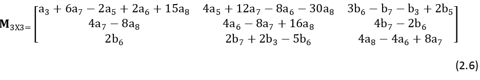
2.3 Mueller matrix

From the Fourier amplitudes a0, (an, bn) of Table 2.1 the 3Х3 Mueller matrix 𝐌3Х3 can

constructed as follows:

𝐌3Х3=

a3+ 6a7− 2a5+ 2a6+ 15a8 4a5+ 12a7 − 8a6− 30a8 3b6− b7− b3+ 2b5

4a7− 8a8 4a6− 8a7+ 16a8 4b7− 2b6

2b₆ 2b₇+ 2b₃− 5b₆ 4a₈− 4a₆ + 8a₇

(2.6)

It can thus be seen from the above that under ideal conditions the Mueller matrix elements can

be expressed as linear combinations of the measured Fourier coefficients of the detected

21

CHAPTER 3

OFFSETS AND IMPERFECTIONS

3.1 Introduction

The original PSA arrangement [2] gives us the partial 3x3 Mueller matrix. In order to

determine the absolute Mueller matrix elements, we need to measure i0. This can be done by

removing the sample and setting the polarizer and analyzer azimuth 0 and π/4, respectively.

This is the so called straight-through configuration as the optical arrangement falls in a straight

line.

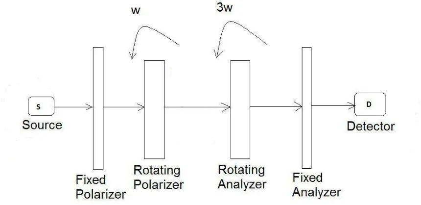
In the modified arrangement we also remove the sample and generate the

straight-through configuration. Parameters that represent the deviations from the ideal case are

introduced gradually and the imperfection parameters are determined in terms of the Fourier

22

Fig 3.1. Straight through configuration: the sample is removed and all optical elements are in line.

3.2 Fourier analysis and determination of imperfection parameters from Fourier coefficients

We now analyze the case where the sample is removed which enables us to measure 𝑖0

directly. In this setting the polarizer and the analyzer come in a straight-through position with

the fixed polarizer azimuth set at P’= 0 and the fixed analyzer azimuth at A’. The Mueller matrix

of the sample thus becomes the identity matrix. The result for such an arrangement is obtained

as a Fourier series given by,

𝑖₀= a0 + 8n=1(ancos(nω′t) + bnsin(nω′t)), (3.1)

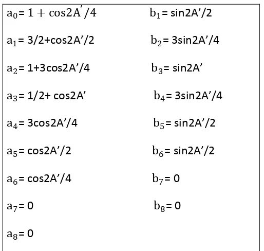
23

a₀= 1 + cos2A′/4 b1= sin2A’/2

a₁= 3/2+cos2A’/2 b2= 3sin2A’/4

a2= 1+3cos2A’/4 b3= sin2A’

a3= 1/2+ cos2A’ b4= 3sin2A’/4

a₄= 3cos2A’/4 b5= sin2A’/2

a₅= cos2A’/2 b6= sin2A’/2

a6= cos2A’/4 b7= 0

a₇= 0 b8= 0

a₈= 0

Table 3.1. Fourier coefficients with straight-through configuration

and simple case of fixed analyzer azimuth A’

We now consider the same straight-through configuration but introduce phase angles

for the rotating polarizer and analyzer. So, let

P=ωt + β and A=3ωt + α (3.2)

while the fixed analyzer azimuth remains A’.

The final equation that we get by calculating i= ГFA𝐌A𝐌S𝐌P𝐒FP where 𝐌S is identity matrix, is

given by,

i= [1+cos(2P)+cos(2A)cos(2A’)+cos(2A)cos(2P)cos(2A’)+sin(2A)sin(2A’)+sin(2A)cos(2P)sin(2A’)]

24

Substitution of A and P from Eqn. (3.2) into (3.3) a Fourier series with coefficients

(a0, a1. . a8, b1. . b8) given in Table 3.2 is obtained.

a0= 1+1₄[cos(2A’)]

a₁=cos(2A

′₎

2 [cos2β+ +

sin (2A′)

2 *sin2β+ + 1

2 *cos2βcos2(α-β)+sin2βsin2(α-β)]+ cos2β

a₂= cos2(α-β) + sin (2A ′₎

2 *sin2(α-β)++

cos (2A′)

2 *cos2(α-β)+ +

cos (2A′)

4 *cos2(α+β)cos2(α-β)+

sin2(α+β)sin2(α-β)] – sin (2A ′₎

4 *cos(α-β)sin2(α+β)-cos2(α+β)sin2(α-β)]

a3= cos(2A’)*cos2α++ sin(2A’)*sin2α+ + 1₂ *cos2βcos2(α-β)-sin2βsin2(α-β)]

a4= cos (2A ′₎

2 *cos2(α+β)++

sin (2A′)

2 *sin2(α+β)++

cos (2A′₎

4 [cos

2_2(α-β)]+sin (2A′)

4 [2cos2(α-β)sin2(α-β)]

a₅= cos (2A ′₎

2 [cos2αcos2(α-β)-sin2αsin2(α-β)]+

sin (2A′)

2 *cos2αsin2(α-β)+sin2αcos2(α-β)]

a6= cos (2A ′₎

4 *cos2(α-β)cos2(α+β)-sin2(α+β)sin2(α-β)]+

sin (2A′)

4 *cos2(α+β)sin2(α-β) -

sin2(α+β)cos2(α-β)]

a7= 0

a8= 0

b1= -sin2β+1₂

[

]+

′₎

2 *cos2αsin2(α-β)-sin2αcos2(α-β)++ sin (2A′)

2 *cos2αcos2(α-β) +sin2αsin2(α-β)+

b₂= -sin2(α-β)+ cos (2A ′₎

2 [-sin2(α-β)++

sin (2A′)

2 *cos2(α-β)++

cos (2A′)

4

*cos2(α+β)sin2(α-β)-sin2(α+β)cos2(α-β)]+ sin (2A ′₎

4 *cos2(α-β)cos2(α+β)+sin2(α-β)sin2(α+β)]

b3= sin(2A’)cos2α- cos(2A’)sin2α - 1₂ *cos2βsin2(α-β)+sin2βcos2(α-β)]

b₄= sin (2A ′₎

2 [cos2(α+β)]-

cos (2A′)

2 *sin2(α+β)+-

cos (2A′)

4 [sin4(α-β)++

sin (2A′)

25

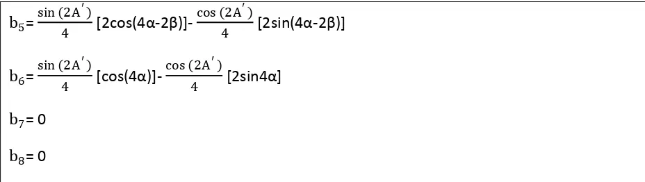
b5= sin (2A ′₎

4 *2cos(4α-2β)+-

cos (2A′)

4 *2sin(4α-2β)+

b₆= sin (2A ′₎

4 *cos(4α)]-

cos (2A′₎

4 *2sin4α+

b7= 0

b8= 0

Table 3.2. Fourier coefficients with the imperfection parameters introduced namely (1) fixed analyzer offset azimuth A’, (2) phase of rotating analyzer α and (3) phase of rotating polarizer β.

The above equations can be solved for the parameters A’, α and β as follows:

4(a0-1) = cos(2A’) (3.4)

The value of A’ from Eqn. (3.4) is used in the following equation to determine α:

a₃+b3 = *cos2α-sin2α+*1/2 + cos(2A’)]+ sin(2A’)*sin2α+cos2α+ (3.5)

Finally the value of α recovered from Eqn. (3.5) is used in the following equation

a₆+b6 = cos (2A

′₎

4 [cos4αcos4β]+ sin (2A′₎

4 *cos4α+sin4α+ (3.6)

to determine β.

Let us now analyze the arrangement taking into consideration the imperfections of the

polarizers. We take out the rotating analyzer from the arrangement and consider the fixed

26

𝐉_FP= 1 0_{0 0} (3.7)

and hence the first column for the Mueller matrix for the same linear polarizer will be

𝐌FP = 1₂[1 1 0 0]T (3.8)

where the T represents the transpose of the matrix.

Fig 3.1. Arrangement without the rotating analyzer in the straight-through configuration.

In certain frequency bands a medium may exhibit both linear birefringence and linear dichroism

concurrently. A linear dichoric retarder is one which has the optic axis of birefringence and

dichroism coincident and parallel with the bounding planar faces. An imperfect polarizer can be

27

refraction n by the complex index of refraction (n-jk) where k is the extinction coefficient of the

medium.

The Jones matrix of the imperfect rotating polarizer can thus be written as

𝐉_P= 1_{0 ρe}0−jδ (3.9)

where

δ=2Πd_λ (n0-ne), ρ =ρ_ρ1

2 = exp[-2πd(ko- ke)/λ+ , ρ<<1 (3.10)

where n0 and ne are the ordinary and extraordinary refractive indices of the medium and

(ke-ko) is called the dichroism of the medium and may be positive or negative.

The Mueller matrix of the rotating polarizer can thus be written as

MP=

1/2 1/2

1/2 1/2 0 00 0

0 0 0 0

ρcosδ ρsinδ −ρsinδ ρcosδ

(3.11)

This is for polarizer azimuth P = 00.

28

M= 1 2 a a x

b 0

m −p b m

0 p

y p q c

(3.12)

where,

a=cos 2P

2

,

sin 2P

2 , c=ρcosδ, p=2b’d, q=-2a’d (3.13)

where a’ and b’ are the terms with rotating analyzer azimuth A instead of P

m= 4ab(1₂-c), (3.14)

x=cos2(2A)(1₂-c)+c, (3.15)

y=4ab(1₂-c) (3.16)

Now the output current is calculated as

i=ГFAMSFP and

Putting P= ωt + β we obtain,

I= ½ + a + cos(2A’)(a+c) + bsin(2A)’ + cos(2A’)cos2(2P)(1/2 - c) + sin(2A’)4ab(1/2 - c) (3.15)

Putting this in Fourier series form we have,

29

Table 3.3. Fourier coefficients in terms of imperfection parameters for the case of ‘missing rotating analyzer’.

From Table 3.3 ρ and β can be calculated as:

2a₀-1 = cos(2A’) (3.16)

b₁= sin (2A′)

2 ( a1 a0 –

sin (2A′_{)sin 2β}

2a0 ) - a0sin2β (3.17)

2b₂= (1

2 - ρcosδ sin(2A’)cos4β – cos(2A’)sin4β (3.18)

The value of A’ is calculated from Eqn. (3.18) and using that in Eqn. (3.19) the value of β can be

obtained. Substitution of these values in Eqn. (3.20) gives the factor ρcosδ.

Now we take the more general case where we include the rotating analyzer in the

straight-through configuration.

2a₀= 1+cos2A’ b₁= sin 2A′

2 cos2β – sin 2β

2 1+cos2A’

a₁= cos 2β

2 (1+cos2A’ + sin 2β

2 sin2A’ b2=

sin 2A′_{cos 4β} 2 (

1

2 - ρcosδ –

cos 2A′sin 4β

2 ( 1

2 - ρcosδ

a₂= cos 2A′cos 4β

2 ( 1

2 - ρcosδ +

sin 2A′_{sin 4β} 2 (

1

30

Fig 3.2. Straight-through arrangement with ideal fixed components and imperfections taken into account in the rotating elements.

The output current equation is given by,

i_D = ГFA𝐌A𝐈S𝐌P𝐒FP (3.21)

where Is is the identity matrix. The rotating analyzer is assumed to be imperfect and the fixed

analyzer offset is A’.

31

a0= 1₄ + c2cos(2A’)+ (1₂ - c)cos(2A’)(c + 1₄ (1₂ - c)) b1= sin (2A

′₎

4 - ( 1 2 - c)

sin (2A′)

4

a₁= cos (2A₂ ′)(1₂ - c) + 1₄ + ₃₂5(₂1 - c) b₂= sin (2A₈ ′) - 1₂(1₂ − c)2 sin (2A′) 2 +

sin (2A₄ ′)(1₂ - c)

a₂= cos (2A₈ ′)+ 1₄ + 1₂(1₂ - c)c.cos(2A’) + 1₄(1₂ − c)2_{cos(2A’) +} d2

2(sin(2A’)-cos(2A’))

a3= cos (2A

′₎ 4 + c 2+ 1 4( 1

2 - c) b3=

sin (2A′) 4

a₄= cos (2A₈ ′)+ (1₂ − c)2 cos (2A′) 4 -

d2

2 (sin2A’-cos2A’ b4=

sin (2A′₎

8 + ( 1 2 − c)

2 sin (2A′) 2

a5= ₃₂3(1₂ - c) – cos (2A

′₎

8 ( 1

2 - c) b5=

sin (2A′) 8 (

1 2 - c)

a₆= 1₂(1₂ - c)cos(2A’)(c+1₂(1₂ - c)) b₆= sin (2A₄ ′)(1₂ − c)2_{+ c.}sin (2A′) 8 (

1 2 - c)

a₇= cos (2A₈ ′)(1₂ - c) b₇= - sin (2A₄ ′)(1₂ - c)

a8=0 b8= 0

Table 3.4. Dependency of the Fourier coefficients in terms of the parameters A’, ρ and δ for the full straight- through configuration considering only the fixed polarizer azimuth to be 0°

From Table 3.4 ρ and A’ are overdetermined as:

2b_b5

3 = (

1

2 - c) (3.22)

4b3= sin(2A’) (3.23)

The value of (1₂-c) and sin2A’ can now be used to get ρ and δ as

cos(2A’)= 3b5−16b_4b 3a5

5 (3.24)

c= ρcosδ= b3_2b−4b5

32

a₄= 3b5−16b_16b 3a5

5 (

1 2+4

b52

b32)-

d2 2 (4b3+

4b3a5

b5 -

3

4) (3.26)

The Eqns. (3.24) to (3.26) establish the relation between the imperfection parameters and

Fourier coefficients of the detected signals. Thus we can determine each of the offset and

imperfection parameters in terms of the measured Fourier coefficients. These parameters are

then used to obtain the Mueller matrix elements as discussed in Chapter 4. If the experimental

results to the Fourier series are available for the above discussed cases, the solution of the

introduced unknowns can be determined accommodating all the equations using the non-linear

33

CHAPTER 4

DETERMINATION OF MUELLER MATRIX ELEMENTS

4.1 Introduction

After the determination of the offset and imperfection parameters from the straight-

through configuration as described in Chapter 3 we now reintroduce the sample between the

rotating polarizer and rotating analyzer. The sample’s Mueller matrix elements are mij

(i,j=0,..,3).

We derive the equation of the detector signal and from there Mueller matrix elements in terms

34

Fig 4.1. Full arrangement where the sample is introduced between the rotating components and all the imperfection parameters are considered.

4.2 Fourier coefficients in terms of imperfection parameters

The Fourier coefficients are shown below in terms of the Mueller matrix elements and

the parameters A’, c and d where,

c=ρosδ (4.1)

35

a₀=m00+m10[cos 2A′₁₆ (₂1-c)+c₂.cos2A’]+m20sin 2A′₄ (7₈+₄c)+m01[(1₂-c)+c₂]+m11[3cos 2A′₁₂₈ (1₂− c)2+ c.cos 2A′₄ (1₂-c)+

c2_cos2A’++m

21[sin 2A′₁₆ (1₂-c)-sin 2A′₁₂₈ (₂1− c)2+c.sin 2A′₂ (7₈+c₄)]

a₁=m10[cos 2A′₁₆ (1₂-c)+c.cos 2A′₂ ]-m20sin 2A′₁₆ (1₂-c)+m₄01+m11[cos 2A′₁₆ (1₂-c)+c.cos 2A′₂ ]+m21sin 2A′₄ +m02sin 2A′₄ (1₂-c)+

m₁₂sin 2A′

8 ( 1

2-c)+m22[ cos 2A′

8 ( 1 2-c)+(

1

2-c)]+m32.d.(sin2A’-cos2A’)( 1

2-c)+m23 cos 2A′

32 .d.( 1 2-c)-m21

sin 2A′ 16 (

1 2-c)

a₂=m00[1₄+cos 2A′₈ ]+m₈10+m01cos 2A′₈ +m₈11+m02sin 2A′₈ +m₈22+m32.d₄(sin2A’-cos2A’)+m03.d.sin 2A′₄ +m23.d₄+

m₃₃.d₂2(sin2A’-cos2A’)

a3=m00cos 2A′₄ +m₄10+m20sin 2A′₄ +m01[3os 2A′₃₂ (1₂-c)+c.cos 2A′₂ ]+m11[(1₂-c).₃₂3+c₂]

a4=m00cos 2A′₈ +m₈10+m01cos 2A′₈ +m₈11-m02sin 2A′₈ +m12sin 2A′₈ (1₂− c)2+m22[cos 2A′₈ (1₂− c)2-1₈]-

m₃₂.d₄(sin2A’-cos2A’)-m03sin 2A′₈ .d-m23.d₄-m33.d 2

2(sin2A’-cos2A’)

36

m₂₂[cos 2A′₈ (1₂-c)-1₄(1₂-c)]+m₄32(1₂-c)-m23.d.cos 2A′₃₂ (1₂-c)

a₆=m10cos 2A′₁₆ (1₂-c)-m20sin 2A′₁₆ (1₂-c)+m₁₆01(₂1-c)+m11[cos 2A′₃₂ (1₂− c)2+c.cos 2A′₈ (1₂-c)+c.cos 2A′₈ (1₂-c)]+

m₂₁[sin 2A′₁₆ (1₂-c)-sin 2A′₃₂ (1₂− c)2-c.sin 2A′₈ (1₂-c)]

a₇=cos 2A′₃₂ (1₂-c)[m10+m11]-sin 2A′₃₂ (1₂-c)[m20+m21]

a8= -m12sin 2A′₈ (1₂− c)2-m22cos 2A′₈ (1₂− c)2

a₉=m01cos 2A′₃₂ (₂1-c)+m₁₆11(1₂-c)

a10=0

a₁₁=0

a12=m11cos 2A′₁₂₈ (1₂− c)2-m21sin 2A′₁₂₈ (1₂− c)2

b1=m02[1₄-cos 2A′₈ (1₂-c)]+m12[cos 2A′₁₆ (1₂-c)+c.cos 2A′₂ -1₈(1₂-c)]+m22[sin 2A′₄ -sin 2A′₁₆ (1₂-c)]+m03.d₂+m13cos 2A′₁₆ (1₂-c).d+

m₂₃[d.sin 2A′₂ -sin 2A′₈ (1₂-c).d]

b₂=m00sin 2A′₈ -m20sin 2A′₁₆ (1₂-c)+m30.d₄(sin2A’-cos2A’)+m01sin 2A′₈ +m₈21+m02[1₄(1₂-c)-cos 2A′₈ ]+

m12[cos 2A′₁₆ (1₂-c).c+cos 2A′₁₆ (1₂− c)2-1₈]+m22[sin 2A′₄ (1₂-c)-sin 2A′₁₆ (1₂− c)2]-m03d.cos 2A′₄ -m13.d₄+

m₃₁.d₄(sin2A’-cos2A’)

b3=m00sin 2A′₄ +m30(sin2A’-cos2A’).d₈+m01[sin 2A′₃₂ (₂1-c)+sin 2A′₂ .c]+m21[₃₂1(1₂-c)+₂c]+m₄20+

m31(sin2A’-cos2A’)*(1₂-c).d₂+d.₂c]

b4=m00sin 2A′₈ +m₈20+m30(sin2A’-cos2A’).d₄+m01sin 2A′₈ +m₈21+m31(sin2A’-cos2A’).d₄+m02cos 2A′₈ +

m12[1₈-cos 2A′₃₂ (1₂− c)2]+m22sin 2A′₁₆ (1₂− c)2+m03cos 2A′₄ .d+m13.d₄

b5=m10sin 2A′₈ (1₂-c)+m20cos 2A′₈ (1₂-c)+m11sin 2A′₈ (1₂-c)+m21cos 2A′₈ (1₂-c)+m02cos 2A′₈ (1₂-c)+

37

Table 4.1. Relation between Fourier coefficients and Mueller matrix elements in terms of parameters A’, ρ and δ where the sample is reintroduced

From the Fourier coefficients are the Mueller-matrix elements are determined. Note that the

coefficients of the frequency of 20ωt and 22ωt are equal to zero, i.e., a9, a10, b9 and b10 are

equal to zero.

4.3 Calculation of Mueller-matrix elements

The solutions of the Mueller matrix elements are determined as given below:

m₂₁= 64(b12−a12tan 2A

′₎

sin 2A′_{tan 2A}′_{+cos 2A}′ ₍1 2−c)2.

1 2

(4.3)

m₁₁=a12+

sin 2A ′ (b 12−a12tan 2A′ ) sin 2A ′ tan 2A ′ +cos 2A′ cos 2A ′

4 ( 1 2−c)2.

1 2

m22

=

′_.b 8 1 16 1 2−c 2

.1₂(sin 2A′_{tan 2A}′_{−cos 2A′ )} (4.5)

m₁₂=b8+

sin 2A ′ (a8+2tan 2A′ b8) sin 2A ′ tan 2A ′ −cos 2A′

cos 2A ′ 16 (

1 2−c)2.

1 2

b₇=sin 2A′₈ (1₂-c)[m10+m11]+cos 2A′₈ (1₂-c)[m20+m21]+cos 2A′₃₂ (1₂-c) [m12+d.m13]-sin 2A′₃₂ (1₂-c)[m22+d.m23]

b₈=m12cos 2A′₃₂ (1₂− c)2-m22sin 2A′₃₂ (1₂− c)2

b₉=m01sin 2A′₃₂ (1₂-c)+m₃₂21(1₂-c)+m31₁₆d(1₂-c)(sin2A’-cos2A’)

b₁₀=0

b11=0

38

m₀₁=

a9−1a12+ b12−a12tan 2A′ tan 2A′ 8 12−c (sin 2A′ tan 2A′ +cos 2A′ )

cos 2A ′ 16

1 2−c .

1 2

By substitution of Eqn. (4.3) and Eqn. (4.4) in

a7=cos 2A′₁₆ (1₂-c).1₂[m10+m11] - sin 2A′₁₆ (1₂-c).1₂[m20+m21] (4.8)

and the values of Eqn. (4.3) and Eqn. (4.4) again in

a6=m10cos 2A′₁₆ (1₂-c)-m20sin 2A′₁₆ (1₂-c)+m₁₆01(₂1-c)+m11[cos 2A′₃₂ (1₂− c)2+c.cos 2A′₈ (1₂-c)+c.cos 2A′₈ (1₂-c)]+

m₂₁[sin 2A′₁₆ (1₂-c)-sin 2A′₃₂ (1₂− c)2-c.sin 2A′₈ (1₂-c)] (4.9)

we obtain the values of m10 and m20.

Further the value of m00 can now be calculated from the equation:

a₃=m00cos 2A′₄ +m₄10+m20sin 2A′₄ + m01[3cos 2A′₃₂ (1₂-c)+c.cos 2A′₂ ]+m11[₃₂3(1₂-c)+c₂] (4.10)

where the only unknown is m00.

Further from

b₉= m01sin 2A′₃₂ (1₂-c)+m₃₂21(1₂-c)+m31(sin2A’-cos2A’).₁₆d.(1₂-c) (4.11)

39

Also since the equation for b3 in Table 4.1 has only m30 as the only remaining unknown, it can

be easily determined as well.

Let us now write the rest of the equations in terms of the remaining unknown parameters.

b1= f(m02, m03, m13, m23) (4.12)

b2= f(m02, m03, m13) (4.13)

b4= f(m02, m03, m13) (4.14)

b5= f(m02, m13, m23) (4.15)

a1= f(m02, m32, m23) (4.16)

a2= f(m02, m32, m03, m23, m33) (4.17)

a₄= f(m02, m32, m03, m23, m33) (4.18)

a5= f(m02, m32, m23) (4.19)

In equations (4.12), (4.14), (4.15), (4.16) and (4.19) we have 5 unknowns of m02, m32, m23,

m₀₃, m13. These can be evaluated using simple algebraic calculations or using determinant

method. Using the above solutions and equation (4.17) or (4.18) we can determine m33 as well.

Thus resulting Mueller matrix parameters are thus determined in terms of the Fourier

40

V SUMMARY

Mueller matrix has important practical applications. One of them is to determine the

change in properties of a sample when placed in a polarizer-sample-analyzer (PSA)

arrangement. The general PSA arrangement is modified in this case by adding fixed polarizer

and analyzer at both ends of the optical train. Simple analysis of this structure gives us the 3x3

block of Mueller matrix of the sample when every optical device is considered to be ideal.

Deviations from ideality are accounted for through the introduction of the azimuthal

offsets and component imperfections. Operation in the straight-through configuration permits

the measurement of these imperfections and offsets from Fourier analysis of the detected

signal. This gives us an estimate of imperfection parameters and their effects in deviation from

the ideal case.

Finally, when the sample is reintroduced and the full Mueller matrix elements are

obtained in terms of the imperfection parameters and the Fourier coefficients of the detected

41

VI FUTURE WORK

The work presented here is theoretical and remains to be applied to an actual

laboratory instrument. The arrangement if realized in a laboratory can be useful in the

determination of the Mueller matrix elements of the sample in the presence of component

imperfections and thus will help us formulate an error analysis that links theoretical and

experimental results.

The error analysis can also further be developed by using the systematic error-

propagation method in which the calculation is done by evaluating the Jacobian matrix that

relates errors δmij of the Mueller-matrix elements of the sample to imperfection parameters

that propagate through the Fourier coefficients δao, δa2n, and δb2n. A similar work was done

using rotating compensators showing the influence of each optical element on the acquired

parameters [6].

The determination of Mueller matrix elements in practical laboratory experiments can

be used to analyze the sample in between for various factors such as change in properties and

can be helpful in various medicinal purposes such as defining the interconnection between

42

REFERENCES

[1] R.M.A. Azzam and N.M. Bashara, Ellipsometry and Polarized light (Elsevier North-Holland,

Amsterdam, 1977 and 1987).

[2] R.M.A. Azzam, Optics Communications 25, 137 (1978).

[3] P.S. Hauge, J. Opt Soc. Am. 68, 1519 (1978).

[4] David S. Kliger, James W. Lewis, Cora E. Randall, Polarized Light in Optics and Spectroscopy

(Academic Press, 1990).

[5] Serge Huard, Polarization of Light (Wiley, New York, 1997).

[6] Laurent Broch, Aotmane En Naciri, Lue Johann, Systematic Errors for a Mueller matrix dual

43

VITA

Shibalik Chakraborty was born in Calcutta, West Bengal, India. He completed his studies

from Ramjas School, R.K.Puram, New Delhi, India in 2002. He then received his Bachelor of

Technology in Electronics and Communication Engineering from Bengal Institute of Technology

under the West Bengal University of Technology, Calcutta, India in 2007. Since August 2007 he

has been pursuing his Master of Science Degree in Electrical Engineering at the University of