Volume 8 - Article 3 | Pages 61–92

in the population sciences published by the Max Planck Institute for Demographic Research Konrad-Zuse Str. 1, D-18057 Rostock · GERMANY www.demographic-research.org

DEMOGRAPHIC RESEARCH

VOLUME 8, ARTICLE 3, PAGES 61-92

PUBLISHED 11 February 2003

www.demographic-research.org/Volumes/Vol8/3/

DOI: 10.4054/DemRes.2003.8.3

Research Article

Bayesian spatial analysis of demographic

survey data:

An application to contraceptive use

at first sexual intercourse

Riccardo Borgoni

Francesco C. Billari

1 Introduction 62

2 Data: Geo-referenced FFS 63

3 Methods: Why Bayesian inference? 67

3.1 A Bayesian spatial model 68

3.2 Monte Carlo Markov Chain inference 70

4 Application to contraceptive use: methodological aspects and results

72

4.1 Monte Carlo Markov Chain setup 72

4.2 Results 72

4.3 Is there a problem with standard multilevel modeling approaches?

76

5 Conclusion and future developments 77

6 Acknowledgements 78

Notes 79

References 82

Appendix 1. Identification issues 86

Research Article

Bayesian spatial analysis of demographic survey data:

An application to contraceptive use at first sexual intercourse

Riccardo Borgoni 1

Francesco C. Billari 2

Abstract

In this paper we analyze the spatial patterns of the risk of unprotected sexual intercourse for Italian women during their initial experience with sexual intercourse. We rely on geo-referenced survey data from the Italian Fertility and Family Survey, and we use a Bayesian approach relying on weakly informative prior distributions. Our analyses are based on a logistic regression model with a multilevel structure. The spatial pattern uses an intrinsic Gaussian conditional autoregressive (CAR) error component. The complexity of such a model is best handled within a Bayesian framework, and statistical inference is carried out using Markov Chain Monte Carlo simulation.

In contrast with previous analyses based on multilevel model, our approach avoids the restrictive assumption of independence between area effects. This model allows us to borrow strength from neighbors in order to obtain estimates for areas that may, on their own, have inadequate sample sizes. We show that substantial geographical variation exists within Italy (Southern Italy has higher risks of unprotected first-time sexual intercourse). The findings are robust with respect to the specification of the prior distribution. We argue that spatial analysis can give useful insights on unmet reproductive health needs.

1 _{Department of Social Statistics, University of Southampton, Highfield, SO17 1BJ, Southampton UK.}

E-mail [email protected] .

2 _{Istituto di Metodi Quantitativi, Università Bocconi, viale Isonzo 25, I-20135 Milano, Italy.}

1. Introduction

In the literature on potential health risks caused by sexual behavior, a particular emphasis is placed on the behavior of adolescents. Adolescents are more likely to contract sexually transmitted diseases (STDs), including HIV/AIDS. Adolescents also have a higher risk of unplanned pregnancies (Kotckick et al., 2001). Consequently, adolescent sexual behavior has been considered one of the fundamental factors for the study of health risks among young people. This is mainly due to the fact that half of all new cases of HIV infections involve young people between 15 and 24 years of age (UNFPA, 2000). Also, the definition of risk behavior is often linked with sexual activity at a particularly early age (Duberstein Lindberg et al., 2000), but attention is also being placed on the use of contraceptive methods at first-time sexual intercourse (Hogan et al., 2000). Ku and collaborators (Ku et al., 1994) have also shown that the use of contraception one’s initial experience with intercourse has a decisive influence on future contraceptive decisions.

In this paper we analyze data from Italy. In this country, young adults tend to wait to have sexual intercourse considerably longer than their counterparts in other Western countries do (Bozon and Kontula 1997; Cazzola 1999; Ongaro 2001). Our attention is directed towards the reproductive health risks of young people who do not use contraceptive methods at first sexual intercourse. Obviously, this indicator needs to be studied in a multi-dimensional context and may be insufficient when considered on its own. More precisely, the study of risk connected with behavior is flawed when the contraceptive method is not known, as the method may not be suitable for the prevention of STDs and/or pregnancy. This is a concern particularly in Italy where traditional contraceptive methods are still used, even by adults (Note 1) (Bonarini 1999; Spinelli et al., 2000). Because of the limits of available data, this study concentrates on the non-use of contraception at first-time sexual intercourse as a risk indicator, not on different types of birth control methods. This indicator will provide an underestimated risk measure of being exposed to pregnancy (because even when birth control is used, the method involved may not be fully effective), and an even more underestimated risk measure for the exposure to STDs (even effective contraceptive methods such as oral contraceptives do not provide protection against STDs) (Note 2). The indicator may however overestimate risks because especially when first sexual intercourse takes place after first marriage, non-contraception may be a choice, although first sexual intercourse in Italy for recent cohorts is almost completely detached from marriage (Ongaro, 2001).

contraceptives are important contextual characteristics in this regard (Brewster et al. 1993; Billy et al. 1994; Teitler and Weiss 2000). This speaks to the importance of geo-referencing individual-level data. Italy is a particularly interesting case for scholars interested in studying geographical differentials, as social and historical heterogeneity within the country corresponds, to a wide extent, to geographical heterogeneity. Throughout Italy, for example, the age at which people have sexual intercourse for the first time varies widely, especially for women (Billari and Borgoni 2002; Ongaro 2001). Mapping territorial influence is also important because any potential policy intervention for risk reduction is more effective when planned at a local level, as in any Western country. With reference to the United States, Teitler and Weiss (2000) found educational context to be of great importance. Furthermore, Mauldon and Luker (1996) showed that contraceptive education makes it one-third more likely that contraception will be used at first-time intercourse, and that condoms will be the method used. The absence of official statistics on the subject creates problems both in terms of measurement and statistical appraisal of reproductive health risks (with the exception of voluntary abortions). In these cases, survey data becomes extremely useful. Furthermore, if one wants to take into account the importance of spatial distribution, one should apply adequate mapping techniques. Such techniques have to be suitable in terms of controlling for sample variability, possibly by exploiting the data’s geographical distribution and the differential spatial incidence of the phenomenon of interest.

This paper proposes methods for the study of spatial distribution in Italy pertaining to the non-use of contraceptives at first-time sexual intercourse by studying the data provided by the Fertility and Family Survey. More precisely, with a spatial statistical model featuring a Bayesian approach, we produce maps at the provincial level. The paper is structured as follows: Section 2 provides an introduction of the data studied. The methodological approach and estimate methods are given in Section 3. The application and results are given in Section 4, and Section 5 contains some concluding remarks. The appendix provides further diagnostics and sensitivity analysis of the MCMC inference.

2. Data: Geo-referenced FFS

Activities Unit (PAU) of the United Nations Economic Commission (UN/ECE) with the intent of collecting comparative information on an international scale.

The sampling strategy, which was created by the National Statistical Institute (ISTAT), is described in detail by Zannella et al. (1997). The survey has a three-stage design, (municipality, electoral section, and individual) and the sample comprises 6,030 individuals, with two independent samples for men and women. More precisely, 4,824 women and 1,206 men born between 1946 and 1975 were interviewed. The interviews were carried out between November 1995 and January 1996 and contained questions pertaining to a series of bio-demographic events. The age of the respondents when these events were experienced was also registered (Note 3).

For the following analysis, we select the subset of individuals who had experienced sexual intercourse. The vast majority of the sample, 5,279 individuals, is included in this subset. Furthermore, all of the respondents whose answer on whether they had experienced sexual intercourse was missing are excluded from the data set (95 cases). The data is considered to be reliable and of good quality by cross-validation with other surveys (Cazzola 1999). In general, data on retrospectively-reported contraceptive use at first intercourse are of sufficiently high reliability in a wide variety of contexts (Wilder 2000). In what follows, we only differentiate between respondents who had used contraception during their initial sexual intercourse experience and those who had not used any contraceptive method. We include cases in which respondents answered "don’t know" on the use of contraception (24 cases) as part of the set of those who had not used any contraception. We thus assume that in absence of explicit reporting of contraceptive use, contraception was not used.

In order to study where respondents lived when they had their first sexual intercourse, we use the place of main residence during the first fifteen years of his/her life (Note 4). This may not have been the respondent’s actual hometown, but we assume that it is a fair reflection of the environment in which the first sexual intercourse was experienced. Individuals living abroad at age fifteen and individuals who did not indicate any residence location are excluded. The municipal data are then aggregated at the provincial level. Given the methodological focus of the present work, we limit our attention exclusively to the sub-sample of women. Finally, cases in which age at first sexual intercourse was not given are excluded from the analysis (32). The final data set includes 4,006 female cases. Among them, 47.6% used some contraceptive methods during their first sexual experience. The sample distribution across age and cohorts is reported in table 1.

cases). This results in a wide variability of the summary statistics, like relative frequencies, in those provinces with few observations.

Table 1: Sample size and percentage of contraceptive use by age at first

intercourse and cohort

Number of women Percentage of contraceptive use

Cohort Cohort

Age at first

intercourse 1946-55 1956-65 1966-76 total 1946-55 1956-65 1966-76 total

under 18 193 388 341 922 35.8 51.8 63.9 52.9

18-20 549 643 577 1769 35.9 44.2 72.1 50.7

21-24 416 289 234 939 28.4 38.4 65.4 40.7

over 25 193 139 44 376 32.1 40.3 52.3 37.5

total 1351 1459 1196 4006 33.0 44.7 67.7 47.6

a) b)

Figure 1: Sample size (a) and contraceptive use counts (b)

0 - 3 3 - 8 8 - 14 14 - 25 25 - 175

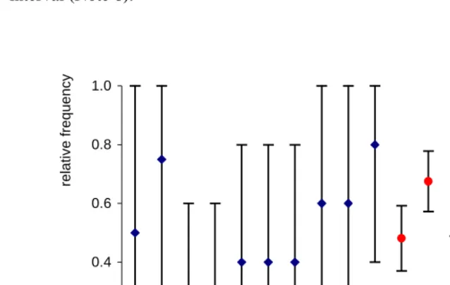
In Figure 2, we show the empirical probabilities for the 8 provinces with the largest sample size (more than 78 units, which is approximately the upper decile of the distribution of the number of observations across provinces) and for the 10 provinces with the smallest sample size (Note 5) (less or equal to 5, approximately the first decile of the distribution of the sample size across provinces) along with their 95% confidence interval (Note 6).

♦ Smaller sample size

•

Figure 2: Frequency of contraceptive use for the provinces with more than 78

observations and less than 5

The map in Figure 3, where observed percentages of contraceptive use are depicted across provinces, already shows a spatial pattern. The following analysis thus aims at using a model that borrows strength from neighbors in order to obtain estimates for areas that may, on their own, have inadequate sample sizes.

0.0 0.2 0.4 0.6 0.8 1.0

NO CZ MC CB PI RI SR GR NU LC BZ GE LE BA _TO MI NA RM

relat

ive f

Figure 3: Relative Frequency of contraceptive use by provinces

3. Methods: Why Bayesian inference?

This section describes the statistical techniques employed; the results are analyzed in detail in Section 4. We use a Bayesian computational approach to statistical inference. This approach makes use of simulation to estimate the posterior distribution of parameters, that otherwise cannot be estimated using standard techniques.

Let O denote the observed data, β the parameter of a model for the data, L(O|β) the

likelihood function of the model, and π(β) the prior distribution which conveys past

knowledge of the parameter β , or the absence of such past knowledge in case of prior distributions with high variability. In Bayesian inference, the posterior distribution,

π(β|O)∝ L(O|β)×π(β), links the assumptions made (the prior distribution) with the

empirical evidence (the likelihood). The goal is to use the characteristics of this distribution (say the mean or the quantiles) to make inferences about β. This approach can be extended to multivariate contexts where β becomes a vector of parameters. Because the parameters are themselves random variables, it is natural to deal with them in a hierarchical way. This means that we are assuming that their distribution may

depend on other parameters, called hyperparameters. These hyperparameters are also random variables with their own prior distributions, called hyperpriors. Such hierarchical thinking helps to understand multiple parameter problems to develop computational strategies and, in practice, to provide enough parameters to deal with complex, hierarchical, data structures (Gelman et al. 1995).

The derivation of any posterior quantity requires evaluation of integrals of the form ∫ξ(β)π(β|O)dβ, for some function ξ(β). Direct integration of this expression is

usually problematic both in analytic and numerical terms. In order to overcome this problem we use the approach known as Markov Chain Monte Carlo (MCMC). MCMC is used to indirectly obtain the posterior distribution: given a sample generated from the posterior distribution, the characteristics of the probability density function are approximated using the sample counterparts. The key of MCMC is to simulate a Markov process whose stationary distribution (the distribution which the transition distributions converge to) is the posterior we are interested in. The simulation has to iterate long enough so that the distribution of the last generated draws is sufficiently close to the posterior distribution.

A full discussion of the advantages and the features of Bayesian modeling and MCMC is, however, far beyond the scope of this paper. The reader may refer, for instance, to Congdon (2001) for an applied perspective, and to Gelman et al. (1995) and Gilks et al. (1996) for a more formal presentation.

We now give a description of the statistical model we used, and we describe the estimation algorithms used in the inferential procedures based on the MCMC approach.

3.1 A Bayesian spatial model

words, we can expect the effects within adjacent areas to be correlated. In section 4.3, we return to the problems arising when one does not consider this type of correlation.

The dependent variable, Y, is dichotomous, where the value 1 represents the respondent’s use of a contraceptive method at first intercourse (0 otherwise). The probability assumption we make is that Y follows a p-mean Bernoulli distribution, and that p is linked to a linear predictor through a logit link function. To model spatial patterns, we add two random variables to the linear predictor. The first random variable,

U, is assumed to be independently and identically distributed for all areas (the unstructured component). The second random variable, S, represents a spatial process

(the structured component). The model is formally specified as follows:

G

g

S

U

X

p

)

’

1

,

,

(

logit

=

β

+

+

=

L

where G stands for the number of areas taken into consideration (in our case the number of Italian provinces totaling 103) and the subscript gi refers to the generic i-th sample

unit in the province g.

Hereafter, the β’s are referred to as fixed effects and the spatial components as random effects. We should keep in mind that in a Bayesian framework all the

parameters of the model are random variables. Unlike in the frequentist tradition, the term ‘fixed’ means that no higher hierarchical level is present beyond the assumed prior, while the term 'random' means that a further prior (called hyperprior) is elicited for the parameters (the so called hyperparameters) of such distributions (Gelman et al. 1995).

Regarding the unstructured component, we assume that the vector U’={U1 ,…, UG}

follows a normal prior distribution with a vector of 0 mean, and a variance and co-variance matrix 2I (with I being identity matrix and 2>0 unknown). For the structured component S’={S1 ,…, SG}, we assume that the prior is represented by a Markov

Gaussian field or conditional Gaussian autoregressive model (Besag et al. 1991). In this case, therefore, with S-g indicating the vector of the effects excluding that of

the g-th location, we assume that:

)

,

(

~

|

g r

r gr g

g

S

N

w

S

S

∑

τ

where w gr and g are defined in terms of the precision matrix. More specifically, we

each adjacent area and a 0 weight otherwise. The mean and the variance are given respectively by:

g g r

r g

g

S

S

m

S

E

(

|

)

∑

/

∂ ∈

−

=

, and

Var

(

S

|

S

)

/

m

τ

=

− (2)

which are expressions that make the model’s Markov structure clear.

The rationale behind this hypothesis is that a spatial effect is usually a surrogate of many unobserved influential factors. Some such factors may obey a strong spatial structure, while others may act only locally. The two different random processes are supposed to grasp such a double source of randomness.

The structured part of the prior allows us to borrow strength from neighbors in order to make the estimates based on inadequate sample sizes more robust. Accordingly, equation (2) states that the conditional mean of Sg is the average of the

neighboring effects and the variance of the distribution is expected to be smaller the higher the number of the neighbors (Note 7).

Finally, in the model’s third stage, we select prior distributions for the fixed effects and for the hyperparameters. We assume a highly dispersed but proper inverse gamma distribution both for the 2 and for the ² parameter (specifically we used a scale parameter b=1 and form parameter a=0.005 inverse gamma law). As we do not have any specific information about the fixed parameters β, neither concerning their range nor their sign, we have assumed a "diffuse" prior distribution for them that is π(βj) is

proportional to a constant for each regression parameter βj. Our assumptions on prior

distributions give almost all the weight to the likelihood function in the construction of posterior distributions (Note 8). For models such as the one we illustrated identification is a potential problem, and an assessment of a possible under-identification of the problem requires the calculation of model diagnostics. We discuss such problems in a detailed way in Appendix 1.

3.2 Monte Carlo Markov Chain inference

adopted for inference, after the exclusion of an initial number of observations used to let the chain converge (burn-in). For the model adopted in this study, we make the following assumptions:

• conditional on explanatory variables and on the entire set of parameters, observations are independent;

• prior distributions for fixed and random effects and hyperpriors are mutually independent.

Given these assumptions, we denote the number of explanatory variables in the model by K, the conditional distributions generically by π(z|y), and the contribution to

likelihood of the i-th unit in the g area by Lgi (ygi ),i = 1,…, ng (where ng represents the

number of observations in the g-th area). The posterior distribution is then factorized as follows:         β π         τ π τ π         σ π σ π         β ∝ β σ τ π

∏

∏

∏

∏∏

MCMC inference is based, therefore, on sample simulation from each full conditional distribution.

The algorithms used for the MCMC simulations in this paper are described in detail in Fahrmeir and Lang (2001-A), so we provide only a brief description here. We adopt the algorithm proposed by Gamerman (1997) to update the model’s fixed parameter values and those of the random unstructured intercepts. The essential idea behind Gamerman's algorithm is to generate an observation by means of a Metropolis-Hastings algorithm step inside the iterative weighted least squared (IWLS) procedure (Note 9). The algorithm we use for the updating of the structured component (CAR) was originally proposed by Knorr-Held (1999) within the framework of dynamic linear generalized models. This algorithm aims at improving the mixing and convergence of simulated chains by updating, at each iteration, a block of values. (Note 10).

4. Application to contraceptive use: methodological aspects and

results

After giving a brief description of the application’s technical aspects, this section contains a discussion of our results (Note 11). We then compare our results to those that would likely have been obtained by adopting an approach that is common in multilevel statistical models, where the usual assumption is the mutual independence between areas.

4.1 Monte Carlo Markov Chain setup

As indicated in the previous section, the basic idea of MCMC methods is to give an approximation of posterior distribution by means of a sample simulated through a Markov chain. The observations of the Markov chain are thus correlated. In principle, as many authors have observed (e.g. Gelman 1996), no substantial problems arise when considering correlated observations in MCMC inference. Nevertheless, correlation may imply the need for simulating very long chains. In this case, computing the results can become burdensome in terms of calculation. One solution is to use only one observation for each k simulated for inference (this is known as thinning). At the same time, the choice of the k-interval according to the auto-correlation in the chain allows for reduction in the correlation to be found in the sample actually used for inference (Note 12).

4.2 Results

We include as explanatory variables, in addition to the province the respondents lived in up until age 15, the respondent’s age at first sexual intercourse (divided into four categories: 14-17 years old as the reference group, 18-20 years old, 21-24 and over 25 years old), and birth-cohort (divided into three categories: 1946-55 as the reference group, 1956-65 and 1966-75).

contraception, as their odds were 7.8% lower than the 14-17 year old reference group). Regarding cohorts, the relative odds for the 1956-65 cohort is 69.5% higher than the oldest cohort, and the increase in odds for the youngest on the date of the interview (those born 1966-75) increased to 345% compared to the reference cohort. These values confirm the strong differentials in frequency of use of contraception mentioned in the introduction.

Table 2: Fixed effects estimates.

Variable Mean S.D. 1st decile Median 9th decile

Intercept -0.716 0.096 -0.838 -0.715 -0.593

Age 18-20 0.066 0.088 -0.049 0.065 0.181

Age 21-24 -0.081 0.105 -0.210 -0.081 0.052

Age 25 and over 0.003 0.141 -0.177 0.002 0.183

1956-65 cohort 0.528 0.087 0.417 0.528 0.638

1966-75 cohort 1.493 0.093 1.377 1.491 1.615

Note: reference groups: age 14-17 and 1946-55 cohort.

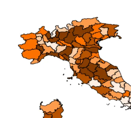
Turning to spatial-related aspects, studied controlling for age and cohort effects, we observe immediately from Figure 4 (a) that there is an increasingly marked effect of the area on the odds of moving from the south to the north of the peninsula. Figure 4 (b) shows in which provinces the effect is either positively or negatively significant, or not significant, meaning that the credibility interval given by the 10th and 90th posterior percentile is above 0, below 0 or it contains 0 respectively.

The maps in Figure 4 show a significant level of heterogeneity at the spatial level between the various Italian provinces which, among other issues, reflects the south-north differentials given by age at initial sexual intercourse found in the same data (Billari and Borgoni 2002; Ongaro 2001).

Considering only the structural variance and not the spatially unstructured component may sometimes be misleading, and may not provide complete information. Only by comparing the two can we understand which areas deviate from the latent structure (in our case, the south-north gradient).

a)

b)

Figure 4: Structured spatial effects (posterior mean) (a) and their credibility

a)

b)

Figure 5. Unstructured spatial effects (posterior mean) (a) and their credibility

values used to delimit this middle group are obtained by adding and subtracting one standard deviation from the overall mean (Note 13). In the unstructured component, no particular trends are evident. In any case, the effects are less relevant in statistical terms than in the structured component. Only eight provinces show significant effects (in terms of an 80% credibility interval). These provinces are highlighted in color in Figure 5 (b), whereas the provinces with non-significant effects are left in white. The provinces of Genoa, Florence, Rome and Sienna stand out as having a positively significant unstructured effect. The provinces with a negatively significant unstructured effect are Caserta, Como, Salerno and Taranto.

Finally, by comparing the distribution of structured and non-structured provincial effects across Italy, we observe that the probability interval given by the 5th and 95th percentiles is equal to (-0.274, 0.329) for unstructured effects and (-0.693, 0.362) for structured effects. To sum up, we conclude that the structured component has more relevance compared to the unstructured component (Note 14).

4.3 Is there a problem with standard multilevel modeling approaches?

In social-demographic research, multilevel statistical models are often used to study spatial clustering problems (Goldstein 1999). With such models, it is usually assumed that the random components at the contextual level are mutually independent. Even though quite common, this assumption is not actually implied by the multilevel approach, so correlated random residuals can also be specified (e.g. Langford et al. 1999). The independence assumption has an inherent problem of inconsistency: if the spatial context matters, it makes sense to assume that areas close to each other are more similar than areas that are far apart. That is, the spatial correlation (i.e. structured component) that we used in the model presented in Section 3.1 applies here as well. In order to emphasize the differences that can be found by adopting this approach in a spatial context and the possible risks involved with the violation of the assumption of independence between aggregated spatial units, we used Model (1) with the non-structured variance component only.

Figure 6: Unstructured spatial effects (posterior mean) for a multilevel model without the structured spatial component

5. Conclusion and future developments

In this paper, we show how it is possible to map a social-demographic risk indicator with the use of data taken from a sample survey that is not directly designed to ensure a coverage of geographical units such as those of interest. The Bayesian computational approach we adopted enables us to provide estimates of parameters in an otherwise too complex model. It also allows us to refrain from the assumption of mutual independence between areas usually imposed in multilevel statistical models.

The absence of information from the survey regarding the type of method used limits the potential of the data studied. Thus, for future reference, it is necessary for this

information to be collected on a geo-referenced basis. One could gain a considerable advantage for spatial analysis with a time-varying geo-referencing of life-course events. In this way, it would also be possible to refer an event to the individual’s context at the time it was experienced.

When considering the structured component, our results reveal how the southern areas have a higher risk at initial sexual intercourse, while the unstructured component indicates that the southern provinces of Caserta, Salerno and Taranto have higher risk factors. We can speculate that less available information and more pressure by the partner against using contraception lie at the root of the territorial differences we find, even though further research is definitely necessary to verify this assumption. As a final caveat, however, we must add that the data provided do not allow the study of the reasons why contraception is not used: therefore, we cannot exclude the fact that there are cases where conception is actually desired in first-time intercourse. More generally, maps enable us to produce "narratives" which are valuable for theory formation (Lesthaeghe and Neels 2002): the mere mapping of a phenomenon does not explain the phenomenon, although it constitutes a strong foundation.

6. Acknowledgements

Notes

1. In the sample we worked with, which is described in detail in section 2, only 47.6% of the female respondents declared that they had used contraception during first-time intercourse. However, this percentage varies considerably across the various cohorts and goes to 33% for the 1946-55 decade birth cohort and to 44.7% for the 1956-65 birth cohort and reaches 64.7% in the 1966-75 birth cohort.

2. On the other hand, in some cases there may also have been a desire for pregnancy at first intercourse, which makes underestimating less serious.

3. The questions relevant to this analysis are given in the ‘Fertility Regulation’ section. The respondents were asked: ‘In order to avoid further questions that may not be relevant, can I ask whether you have ever experienced complete intercourse?’ (possible answers: 'yes', 'no', and 'no answer'). In case of an affirmative reply, the person was asked ‘At what age did you have complete intercourse for the first time?’ (with the possibility of stating ‘no answer’) and ‘On that occasion, was any contraceptive method used?’ (possible answers: 'yes', 'no', 'don’t know', and 'no answer'). Unfortunately, the respondents were not asked what type of contraceptive method they had used, if any; this was investigated and limited to the last 4 weeks before the interview (Bonarini 1999).

4. The following question was asked ‘Where did you live for most of the time until you were fifteen years old?’

5. From the set of those Italian provinces eligible to appear in the picture we exclude three provinces with 0 cases of contraceptive use and one province with one observation only.

6. Given the small sample size, we use Bca bootstrap intervals (Davison and Hinkley 1997).

7. We can suggest a demographic meaning for the formulation of the variance in equation (2). If we assume that behavior is influenced in an important way by the context (in our case by geography), and that spatial autocorrelation helps in capturing such influence, the mere fact of having more neighbors allows one to draw more precise conclusions about the average behavior in a given province.

generalized least-squares (IGLS). The main advantage of the Bayesian approach consists in providing the full posterior distribution, while IGLS produces estimates of spatial residuals and their standard errors, the latter using sample estimates only (Leyland, 2001). On the other hand, the Bayesian approach is much more computationally intensive than the latter.

9. This procedure is usually chosen for the maximum likelihood estimations within the framework of generalised linear models (McCullagh and Nelder 1989).

10. These types of algorithms make considerable computational advantages from the sparse structure of the correlation matrix, and also reflect the adjacent relations between areas For further developments and details on highly efficient calculation methods for the generation of Gaussian Markov fields, see Rue (2001).

11. We conducted the analyses presented in this study using BayesX (Lang and Brezger 2000). BayesX is package for Bayesian data analysis, freely available through the Internet at www.stat.unimuenchen.de. They could alternatively have been conducted with the use of other software products for Bayesian analyses, particularly WinBug (Spiegelhalter et al. 2000). S-Plus functions (Venables and Ripley 2000) were used for the final preparation of the results and for the graphics, whereas the various maps were generated with Arc/View GIS (ESRI 1996).

12. For this reason, we simulated preliminarily a chain of 22,000 iterations (of which 2,000 were used for burn-in), from which we analysed the auto-correlation function. The correlation turned out to be negligible (< 0.15) for lags larger than 25-30 for all the parameters studied in the model, so that in the final simulation a thinning pass of one observation every 30 was used. This final simulation consisted in 95,000 iterations (5,000 for the chain burn-in) of which 3,000 (one out of every 30) were used for final estimations. A diagnostic on the results obtained by the MCMC inference is given in Appendix 2.

13. The middle group thus covers a two-standard-deviation interval, while other groups cover one-standard-deviation intervals.

14. In our analyses, we evaluated the trade-off between S and U in a graphical way, looking at maps and at some summary statistics of the distribution of effects (as in Fahrmeir and Lang, 2001-B). Other more formal approaches are also possible and have been suggested in the literature. For instance, Best et al. (1999) define the quantity

}

)

SD(

)

/{SD(

)

SD(

S

S

+

U

=

References

Besag, J., Koopemberg, C. (1995). "On conditional and intrinsic autoregression",

Biometrika, 82(4): 733-746.

Besag, J., York, J., Mollié A. (1991). "Bayesian image restoration, with two applications in spatial statistics", Annals of the Institute of Statistical

Mathematics, 43(1):1-59.

Best N.G., Arnold R. A., Thomas A. (1999) Bayesian models for spatially correlated disease and exposure data, In Bernardo J. M., Berger J.O., Dawid A. P. and Smith A. F. M. Bayesian Statistics 6, Oxford University Press, 131-156.

Billari, F.C., Borgoni, R. (2002). "Spatial profiles in the analysis of event histories: an application to first sexual intercourse in Italy", International Journal of

Population Geography, 8: 261-275.

Billy, J., Brewster, K., Grady, W. (1994). "Contextual effects on the sexual behavior of adolescent women". Journal of Marriage and the Family, 56: 387-404.

Bonarini, F. (1999). L'uso della contraccezione in Italia: dalla retrospezione del 1979 a quella del 1995-96. In De Sandre, P., Pinnelli, A., Santini, A., editors. Nuzialità e fecondità in trasformazione: percorsi e fattori del cambiamento. Bologna: il Mulino: 395-411.

Bozon, M, Kontula O. (1997). "Initiation sexuelle et genre. Comparaison des évolutions de douze pays européens", Population, 6: 1367-1400.

Brewster, K.L., Billy, J.O., Grady, W.R. (1993). "Social context and adolescent behaviour: The impact of community on the transition to sexual activity", Social

Forces, 71(3): 713-740.

Brooks, S. P., Gelman, A. (1998). "General methods for monitoring convergence of iterative simulations", Journal of Computational and Graphical Statistics, 7: 434-455.

Cazzola, A. (1999). L'ingresso nella sessualità adulta. In De Sandre, P., Pinnelli, A., Santini, A. editors, Nuzialità e fecondità in trasformazione: percorsi e fattori del cambiamento. Bologna: il Mulino: 311-326.

Congdon, P. (2001). Bayesian statistical modelling, Wiley, New York.

De Sandre, P., Ongaro, F., Rettaroli, R., Salvini, S. (1997). Matrimonio e figli: tra rinvio e rinuncia. Bologna: il Mulino.

Duberstein Lindberg, L., Boggess, S., Porter, L., Williams S. (2000). Teen risk-taking: A statistical portrait. Washington, DC: Urban Institute.

Eberly L. E., Carlin B. P. (2000). Identifiability and Convergence Issues for Markov Chain Monte Carlo Fitting of Spatial Models, Statistics in Medicine, 19:2279-2294.

Elliot, P., Wakefield, J. (2001). "Disease clusters: Should they be investigated, and, if so, when and how", Journal of the Royal Statistical Society, Series A, 164: 3-12.

ESRI (1996). Using ArcView GIS, Redlands CA: Enviromental Systems Research Institute.

Fahrmeir, L., Lang, S. (2001-A). "Bayesian Inference for generalised additive mixed models based on Markov random field priors", Applied Statistics, 50: 201-220.

Fahrmeir, L., Lang, S. (2001-B). Bayesian Semiparametric Regression Analysis of Multicategorical Time-Space Data. Annals of the Institute of Statistical

Mathematics, 53: 10-30.

Gamerman, D. (1997). "Sampling from the posterior distribution in generalised linear mixed model", Statistics and Computing, 7: 57-68.

Gelfand A.E., Sahu S.K. (1999). Identifiability, Improper priors, and Gibbs Sampling for generalized linear model. Journal of the American Statistical Association, 94: 247:253.

Gelfand A.E., Carlin B.P., Trevisani M. (2001). On computation using Gibbs sampling for multilevel models. Statistica Sinica, 11: 981:1003.

Gelman A., (1996). Inference and monitoring convergence. In Gilks, W. R., Richardson, S., Spiegelhalter, D. J., editors. Monte Carlo Markov Chain in practice. London : Chapman and Hall: 131-143.

Gelman, A., Carlin, J. B., Stern, H. S., Rubin, D. B. (1995). Bayesian data analysis. London: Chapman and Hall.

Gelman, A., Rubin, D. (1992). "Inference for iterative simulation using multiple sequences", Statistical Sciences, 7:457-511.

Goldstein, H. (1999). Multilevel statistical models. First Internet Edition, http://multilevel.ioe.ac.uk/index.html.

Hogan, D.P., Sun, R., Cornwell, G.T. (2000). "Sexual and fertility behaviors of American females aged 15-19 Years: 1985, 1990 and 1995", American Journal

of Public Health, 90(9): 1421-1425.

Knorr-Held, L. (1999). "Conditional prior proposals in dynamic models", Scandinavian

Journal of Statistics, 26:129-144.

Knox, G. (1989). Detection of clusters. In Elliot, P. editors. Methodology of enquiries into disease clustering. London: Small Area Health Statistic Unit: 17-22.

Kotckick, B.A., Shaffer A., Forehand, R., Miller, K.S. (2001). "Adolescent sexual risk behavior: A multi-system perspective", Clinical Psychology Review, 21(4): 493-519.

Ku, L., Sonenstein, F., Pleck, J. (1994). "The dynamics of young men’s condom use during and across relationships", Family Planning Perspectives, 26(6): 246-251.

Lang, S., Brezger, A. (2000). BayesX, Munich: University of Munich.

Langford, I. H., Leyland, A. H., Rabash, J., Goldstein, H. (1999). "Multilevel modeling of the geographical distributions of diseases", Journal of Royal Statistical

Society, Series A (Applied Statistics), 48: 253-268.

Lawson, A.B. (2001) Statistical Methods in Spatial Epidemiology, New York: Wiley & Sons.

Leyland A.H. (2001) Spatial Analysis. In Leyland, A.H., Goldstein, H. editors. Multilevel modelling of Health Statistics, New York: Wiley: 143-157.

Lesthaeghe R., Neels K. (2000). "Maps, narratives and demographic innovation". IPD-WP 2000-8, Interface Demography, Brussels.

Mauldon, J., Luker, C. (1996). "The effects of contraceptive education on method use at first intercourse", Family Planning Perspectives, 28: 19-24.

McCullagh, P., Nelder, J.A. (1989). Generalised linear models (2nd ed.). London: Chapman and Hall.

Pinheiro J.C., Bates D.M. (2000). Mixed Effects Models in S and S-Plus. Berlin: Springer.

Poirier D. J. (1998) “Revising Beliefs in Non-identified Models". Econometric Theory, 14: 483-509.

Rue, H. (2001). "Fast sampling of Gaussian Markov random fields", Journal of the

Royal Satistical Society Series B, 63: 325-38.

Spiegelhalter, D., Thomas, A., Best, N. (2000). WinBUGS: User manual, http://www.mrc-bsu.cam.ac.uk/bugs.

Spinelli, A., Figà Talamanca, I., Lauria, L., and the European Study Group on Infertility and Subfecundity (2000). "Patterns of contraceptive use in 5 European countries", American Journal of Public Health, 90(9): 1403-1408.

Teitler, J.O., Weiss, C.C. (2000). "Effects of neighborhood and school environments on transitions to first sexual intercourse", Sociology of Education, 73(2), 112-132.

UNFPA (United Nations Population Fund) (2000). Preventing infection-promoting

reproductive heatlh. UNFPA’s response to HIV/AIDS, New York: United

Nations.

Venables, W. N., Ripley, B. D. (2000). S programming, Berlin: Springer.

Wakefield, J. C., Kelsall, J. E., Morris, S. E. (2000). Clustering, cluster detection and spatial variation in risk. In Elliott, P., Wakefield, J. C., Best, N.G., Brings D. J. editors. Spatial Epidemiology: Methods and applications, Oxford: University Press: 128-152.

Wilder, E.I. (2000). "Contraceptive use at first intercourse among Jewish women in Israel, 1962-1988", Population Research and Policy Review, 19: 113-141.

Appendix 1. Identification issues

Identification is an issue in models like the one illustrated in Section 3.1, mostly because of two problems. The first problem concerns the CAR prior: as this prior is defined conditionally, the parameter is uniquely specified only up to an additive constant. This problem is well-known in spatial statistics, and several solutions have been proposed in the literature (i.e. imposing a 0-sum constraint to structured effects as in Besag and Kooperberg, 1995). A second problem concerns the identifiability of the two sources of randomness included in the model, namely the unstructured and structured spatial components. This problem is well described by Eberly and Carlin (2000) in the case of a Poisson spatial regression for aggregate area-level data. In that context, letting Ng be the number of events in the area g, it is usually assumed that Ng is

Poisson-distributed, with expected value Egexp(µg), Eg being a known expected number

of event for the area g and µg the log-rate of the event of interest. The model is specified

as µg=Z’gβ+Sg+Ug where Z is a set of area-level covariates, and S and U are random

effects allowing for overdispersion due to clustering and area-level heterogeneity respectively. Given the system of priors described in section 3.1, an identification problem arises because the number of events Ng cannot possibly provide information

about both Sg and Ug, but only about their sum Wg =Sg + Ug This basically means that

once one reparameterizes the model in terms of (U,W), the conditional distribution

π(ug|ur≠g, w, y), does not depend on the data y. This is known as Bayesian

unidentifiability (Gelfand and Sahu, 1999). Even if the model is affected by Bayesian

unidentifiability, this does not preclude Bayesian learning about the parameter that would require π(ug|y)= π(ug) instead, a stronger condition implying that the marginal

Taking all the above issues into account, the identification problem in such models (Fahrmeir and Lang , 2001-B) is more a data-related problem – how many isolated areas are there, how many observations are there in each area – than a problem connected to the estimation algorithm – which sampler, which starting values, the precise prior values chosen (Eberly and Carlin, 2000). A full analysis of identifiability in models such as the one discussed in Section 3.1 is beyond the scope of the present paper, and this Appendix is only provided to make the reader aware of the problem. Moreover as Eberly and Carlin (2000) and Gelfand et al. (2001) observed, even though the assessment of the effect of over-specification is still somehow possible when fixed values are assumed for the variance parameters (that is the model consists of two levels of hierarchy only) assessing clearly the effect of over-specification becomes much more difficult when hyperpriors on the variance parameters (as we do in the present paper) are used instead.

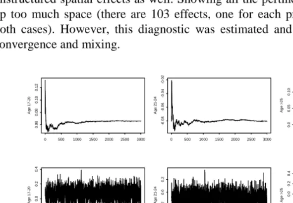
Appendix 2. Diagnostics of MCMC inference

In this appendix, we report diagnostics on the analysis of section 4.2. Although no diagnostic analysis whatsoever can be considered conclusive proof of the validity of inference conducted with the use of MCMC methods, there is no doubt that a study based on this approach cannot avoid considering that inference. Figures A.1 and A.2 report the ergodic averages (first row), the simulated values (second row) and the auto-correlation functions for the 3,000 values used for the inference of the model’s fixed effects. The chain presents a good mixing and a sufficiently quick convergence (even though it has to be considered that the graphs refer to the sampled chain with a 1-out-of-30 thinning). The same type of diagnosis was implemented for the structured and unstructured spatial effects as well. Showing all the pertinent graphs would have taken up too much space (there are 103 effects, one for each province, to be considered in both cases). However, this diagnostic was estimated and showed a very satisfactory convergence and mixing.

Figure A.1: Ergodic means, simulated values and autocorrelation functions of each

parameter of variable "age"

A

ge

17-2

0

0 500 1000 1500 2000 2500 3000

0.06 0.08 0.10 0.12 A ge 17-20

0 500 1000 1500 2000 2500 3000

-0 .2 0.0 0 .2 0.4 c oef. autoc or r.

0 50 100 150 200 250

0.0 0 .2 0.4 0 .6 A ge 21-2 4

0 500 1000 1500 2000 2500 3000

-0 .08 -0.06 -0 .04 -0.02 A ge 21-24

0 500 1000 1500 2000 2500 3000

-0 .4 -0 .2 0.0 0 .2 c oef. autoc or r.

0 50 100 150 200 250

0.0 0 .2 0.4 0 .6 A ge > 2 5

0 500 1000 1500 2000 2500 3000

0.0 0 .05 0 .10 A ge > 2 5

0 500 1000 1500 2000 2500 3000

-0 .4 0.0 0 .2 0.4 c oef. autoc or r.

0 50 100 150 200 250

Figure A.2: Ergodic means, simulated values and autocorrelation functions of the

intercept (first column) and of the 1956-65 and 1966-75 cohort parameters (second and third columns respectively)

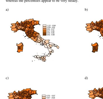
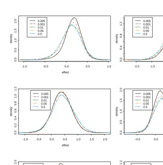
Concerning spatial effects, here we provide a brief sensitivity analysis on the prior distributions. Particular attention is placed on the prior distribution of the CAR model variance parameter, and more informative and proper prior distributions are imposed on the same. In particular, we take distributions of inverse gamma (IG) type into consideration, having a b = 1 scale parameter and form parameter a respectively equal to 0.001, 0.01, 0.05, and 0.5. We can note that the probability mass assigned by each of these distributions to the interval, for example, [0,100] passes from 0.004 for an inverse parameter gamma equal to 1 and 0.001 to 0.89 in case of parameters equal to 1 and 0.5. For each prior distribution, the model is evaluated by implementing a Markov Chain consisting of 95,000 iterations with a 5,000 sample burn-in and a 1-out-of-30 thinning.

The results obtained are given in Figure A.3 for estimated spatial effects, and in Figure A.4 for credibility intervals. In Figure A.3 the mapping composition is obtained by establishing colors according to quintiles. A substantial stability concerning the

c

ons

t

0 500 1000 1500 2000 2500 3000

-0. 8 2 -0. 78 -0. 7 4 c ons t

0 500 1000 1500 2000 2500 3000

-1. 0 -0. 8 -0. 6 -0. 4 c oef . aut oc orr.

0 50 100 150 200 250

0. 0 0 .2 0. 4 0 .6 gen56-65

0 500 1000 1500 2000 2500 3000

0. 52 0. 56 0. 60 gen56-65

0 500 1000 1500 2000 2500 3000

0. 2 0 .4 0. 6 0 .8 c oef . aut oc orr.

0 50 100 150 200 250

0. 0 0 .2 0. 4 0 .6 gen66-75

0 500 1000 1500 2000 2500 3000

1. 50 1. 52 1. 54 1. 56 gen66-75

0 500 1000 1500 2000 2500 3000

1. 2 1 .4 1. 6 1 .8 c oef . aut oc orr.

0 50 100 150 200 250

phenomenon’s spatial trend and concerning the provinces that either do or do not present significant effects (positive or negative) stands out clearly. The prior differences appear to mainly influence the estimates on the tails of the province effect distribution whereas the percentiles appear to be very steady.

a) b)

c) d)

Figure A.3: Structured spatial effects (posterior mean) relative to different priors

(a) IG(1,0.001), (b) IG(1,0.05), (c) IG(1,0.01), (d) IG(1,0.5)

-0.85 - -0.58 -0.58 - 0 0 - 0.24 0.24 - 0.31 0.31 - 0.37 0.37 - 0.44 -1.12 - -0.54

-0.54 - 0.01 0.01 - 0.17 0.17 - 0.31 0.31 - 0.41 0.41 - 0.59

-0.75 - -0.57 -0.57 - -0.01 -0.01 - 0.22 0.22 - 0.29 0.29 - 0.34 0.34 - 0.39

negative effect no effect positive effect

negative effect no effect positive effect

negative effect no effect positive effect

negative effect no effect positive effect

a ) b )

c ) d )

Figure A.4: Credibility intervals of structured spatial effects relative to different

priors: (a) IG(1,0.001), (b) IG(1,0.05), (c) IG(1,0.01), (d) IG(1,0.5)

Figure A.5: Structured spatial effect distributions of six provinces for different inverse

gamma priors (scale parameter equal to 1 and several shape parameter values)

Finally, although no indicator-based diagnostic was implemented for the model parameters (e.g. Gelman and Rubin 1992 and Brooks and Gelman 1998) other than the graphs presented at the beginning of this appendix, the large number of chains analyzed showed a substantial convergence to the values discussed in section 4. This assures us

effect

densi

ty

-1.0 -0.5 0.0 0.5 1.0

0. 0 0 .5 1. 0 1 .5 2. 0 0.005 0.001 0.01 0.05 0.5 effect densi ty

-2.0 -1.5 -1.0 -0.5 0.0 0.5

0. 0 0 .4 0. 8 1

.2 0.0050.001 0.01 0.05 0.5 effect densi ty

-1.0 -0.5 0.0 0.5 1.0 1.5 2.0

0. 0 0 .2 0. 4 0 .6 0. 8 1 .0 1. 2 0.005 0.001 0.01 0.05 0.5 effect densi ty

-0.5 0.0 0.5 1.0 1.5

0. 0 0 .5 1. 0 1 .5 2. 0 0.005 0.001 0.01 0.05 0.5 effect densi ty

-0.5 0.0 0.5 1.0

0. 0 0 .5 1. 0 1 .5 2. 0 2 .5 0.005 0.001 0.01 0.05 0.5 effect densi ty

-1.0 -0.5 0.0 0.5 1.0 1.5