BUFFER CAPACITY IN HETEROGENEOUS MULTICOMPONENT SYSTEMS. REVIEW

BUFFER CAPACITY IN HETEROGENEOUS MULTICOMPONENT

SYSTEMS. REVIEW

Oxana Spinu

*

_{, Igor Povar}

Institute of Chemistry of Academy of Sciences of Moldova, 3, Academiei str., Chisinau MD-2028, Republic of Moldova *e-mail: [email protected]; phone (+373 22) 73 97 36

Abstract. The quantitative basis of the theory of buffer properties for two-phase acid-base buffer systems and for multicomponent heterogeneous systems has been derived. The analytical equations for buffer action with respect to all components for diverse multicomponent systems were deduced. It was found a remarkable relation of proportionality between β_iquantities. It is shown, that the buffer properties in relation to the solid phase components are amplifi ed with an increase of solubility due to protolytic or complex formation equilibria in saturated solutions. It has been established, that the buffer capacities of components are mutually proportional, whereas for heterogeneous systems these relationships depend on the stoichiometric composition of solid phases. The deduced equations can be applied to the assessment of buffer action of the systems “Natural mineral – soil solution”, containing soluble and insoluble chemical species. A number of the important conclusions concerning the investigated buffer systems has been made. The obtained results can be used in various areas of chemical and biochemical researches, especially in soil science, ecological sciences, analytical chemistry, pharmacology, pharmaceutics, medical industry and synthetic organic chemistry

Keywords: buffer action, complex formation, thermodynamic stability, extraction multicomponent system, heterogeneous equilibria.

Received: April 2015/ Revised fi nal: September 2015/ Accepted: September 2015

Introduction

Buffer capacity is an important concept in many areas of science: analytical and electroanalytical chemistry [1], geochemistry [2], biochemistry [3], medicine and pharmaceutical industry [4], water treatment [5], agriculture [6], environment [7], etc. The capacity of buffer systems to oppose (resist) to the variation of their composition (usually to рН changes) by infl uence of external fl uxes of chemical compounds of natural or anthropogenic character, that shift chemical equilibria, is called buffer property, and its effi ciency – buffer action. Despite of an abundance of the information on buffer systems, the quantitative theory of buffer action has been developed only for mono-phase systems [8,9]. The buffer action of mono-phase buffers is usually based on protolytic equilibria between water, a weak acid or base or ampholytic compound and their conjugate pairs [10,11]. The widespread use of buffers as well as the variety of chemical processes and phenomena associated with a certain acidity of solutions explains the constant interest in designing and studying new buffer systems.

Unlike the classical mono-phase buffer systems in which the buffer components are dissolved in a unique phase, in two-phase (heterogeneous) buffers they are distributed between two phases: in aqueous phase and solid (gaseous or liquid) phase. The aqueous (buffer) phase contains all the charged particles and a restricted quantity of electro-neutral species. The solid phase contains in signifi cant quantities only electro-neutral particles and serves as their reservoir by means of which the equilibrium is adjusted and one of parameters of buffer system is maintained constantly [9-18]. The buffer action of two-phase systems is based on the shift of complex equilibria, both homogeneous and heterogeneous in the aqueous phase and between phases, respectively [19-21]. By increasing the acidity of solution the role of simultaneous proceeding protolytic reactions with participation of salt anions increases; with an increase of alkalinity the contribution of complex formation reactions occurring with participation of salt cations amplifi es. Authors [15] have proved that the buffer capacity is a special case of the sensitivity analysis, as a more general theoretical approach, which studies the answer of system to various external perturbations (as for example, the variation of the certain component concentration). We believe that it is more correct to consider, as a potential reservoir of buffer heterogeneous systems, the complex chemical heterogeneous equilibria with participation of solid phases [16]. Unfortunately, so far there are a small number of studies dedicated to the systematic investigations and the development of theoretical aspects of the buffer action for two-phase systems [8,9,14-21]. Besides, in the majority of these studies only the рН – buffer properties of heterogeneous systems were investigated. The concept of “buffer action” helps to fi nd out which reactions control the composition of natural waters, including soil solutions [22-32]. The parameters of buffer action are integrated functions of all the soil chemical components by virtue of their capacity, by means of chemical reactions and sorption-desorption processes, to extinguish or strengthen the effect of entered pollutants [33].

considered in detail. It is proved that the heterogeneous multicomponent systems possess buffer action with respect to all components “i” of acid-base mixtures. Analytical equations for the buffer capacities of two-phase systems with respect to all the components of heterogeneous systems have been deduced. Moreover, it has been shown that the quantities in these systems are reciprocally proportional. In contrast to classical mono-phase buffers, in two-phase buffer systems the maximum buffer capacity β_H occurs when pH_max is equal to pK_d + log(1 + P(HA)), where K_d and P(HA) are respectively the dissociation constant and the repartition constant of the acid between two phases.

Theoretical part

Buffer action of the systems “Mineral – saturated solution”

The buffer action of soil is one of its fundamental physicochemical characteristics. The soil buffer action composes of the buffer action of a set of mineral and organic components and presented by solid, liquid and gaseous compounds. The buffer capacity of soils in relation to chemical compounds is defi ned by the content of chemical elements in the soil solution (the parameter of intensity) and on the content of mobile compounds of these elements in solid phases (the parameter of capacity). The buffer capacity of soils can be discovered by the fact that the increase of amounts of toxic metals (ТМ) is not accompanied by an increase of their content in plants; the different buffer action of the soils in relation to one element is manifested in unequal toxic concentrations for plants [33]. The same soil can possess different buffer action in relation to different metals.

The complexity of the soil solution composition containing mineral phases and a large set of involved chemical compounds determine the possibility of simultaneous chemical reactions along with the capacity of solid phases of minerals to maintain relatively constant the aqueous solution composition [19-21,29-32,34-40]. Under real conditions the buffer action of natural heterogeneous aqueous systems is expressed so as the consumption of any element from solution causes the partial dissolution of solid phases and as a result the composition of the solution is restored.

Currently, extensive information on negative (harmful) transformations of soils, as a result of progressing acid and alkaline loads (in the form of mineral fertilizers, chemicals for protection of plants and industrial emissions dropping out with atmospheric precipitation) has been gathered. Thus, the quantitative assessment of the acid - base buffer action, revealing the degree of infl uence of the systematic use of fertilizers and technogenic pollution by substances of the acid and alkaline nature is an actual problem of the agrology. Besides, the buffer action of soils contains important information on the processes of soil formation (their orientation and intensity) which is used for the soil diagnostics and classifi cation [33].

As a criterion for quantitative assessment of the intensity of buffer action of the studied multicomponent heterogeneous systems, one can use the value of the buffer capacity S

i

 (the superscript index “S” specifi es the presence of solid phases), which can be defi ned as a partial derivative:

) ( 0

0

] ln[

i j C i S i

j

i C

         

  

where 0

i

C and [i] denote the initial (analytical) concentration in mixture and equilibrium concentration of the component “i” of solid phase, correspondingly, the subscript index shows that the initial concentrations of other components of the mixture are maintained constant.

We will examine the process of formation of the sparingly soluble salt of arbitrary stoichiometric composition M_mA_n(S) (M - metal ion, A - anion of salt):

. ] [ ] [ ,

)

(S S m n

n

mA mM nA K M A

M (1)

The following set of possible simultaneous reactions in the saturated solution is taken into account:

] /[ ] ][ ) ( [ ,

) (

2O M OH iH K M OH H i M

iH

M i i i (2)

j

j j

jA K H A A H

H jH

A , [ ]/[ ][ ] (3)

r q

q r q q

rA K MH A M H A

MH rH qA

M , [ ]/[ ][ ] [ ] (4) ].

][ [ ,

2O H OH K H OH

H _w (5)

¦

¦

¦¦

' '

1 0 1 0

0 _{[ ( ) ] [ ]}

i q r

q r j i j M r M M

M C C C iM OH MH A

C ₍₆₎

¦

¦¦

' '

0 1 0

0 _{[ ] [ ]}

l q r

q r l A r A A

A C C C H A qMH A

C ₍₇₎

¦¦

¦¦

¦

1 1 1 1 1

0 _{[ ] [ ] [ ] [ ( ) ] [ ]}

q r q r i j j i l l

H H OH lH A jM OH r MH A

C (8)

The quantity r i

C represents the residual concentration in solution of the ion “i”, e.g. the total concentration of all the species, containing a given ion, while Ci is its molar quantity in the solid phase in 1 L of solution [14-17,41-42].

In the Eq.(8) C_H0 denotes the excess of H+ _{ions in relation to hydroxyl ions in two-phase mixtures (} 0 0 ₎ OH

H C

C . The

square brackets designate the equilibrium concentrations of species in solution.

From the stoichiometric composition of the solid phase, the following ratio is obtained:

n C m CM _ A 

or A _m CM

n C  



(9) On the basis of the written equations it is possible to deduce the formulas for calculating the buffer capacity in relation to any component of the mixture. After a series of transformation, one can fi nally get:

¦¦

¦

¦

¦¦

¦

¦¦

¦¦

¦

¦

¦¦

¦

¦

¦

¸ ¸ ¹ · ¨ ¨ © § ¸ ¸ ¹ · ¨ ¨ © § 1 0 2

0 1 2 1 0

2 2

2 2

1 1 0 1 1

2 2

2

2

1 1 1 1

1 0 1

] ) ( [ ] [ 1 2 ] [ ] [ ] ) ( [ ] [ ] [ ] [ ] [ ] [ ] [ ] ) ( [ i j j i

l q q r

q r l

l i j q r

q r j

i l

q q r

q r r q r i l l j i j S M OH M i A MH n mq n q m A H n m A MH r OH M j A H l OH H A MH rq n m A MH r A H l n m OH M ij E

(10) or 2 2 1 3 _

 S  

M ,

(11) where φ_1,φ₂ and φ₃ denote the following concentration functions:

¦

¦

¦¦

¦

¦

¦

1 1 1 1

1 0 1

1 [ ( ) ] [ ] [ ] [ ]

q q r

q r r q r i l l j i j A MH rq n m A MH r A H l n m OH M ij M

¦

¦¦

¦¦

1 1 0 1 1

2 2

2

2 [ ] [ ] [ ] [ ( ) ] [ ]

l i j q r

q r j

i

lA j M OH r MH A

H l OH H

M (12)

¦¦

¦

¦

_¸¸

¦¦

¹ · ¨ ¨ © § 1 0 2

0 1 2 1 0

2 2

2 2

3 [ ] 2 1 [ ] [ ( ) ]

i j

j i

l q q r

q r

l mq_n MH A i M OH

n q m A H n m M

Similarly, it is possible to prove that, for the buffer capacity towards proton, the following expression is valid: 3 2 1 2 , 0 0 0 ] ln[ M M M E { ¸ ¸ ¹ · ¨ ¨ © § w w S H C C H A M H C (13)

For the buffer capacity towards the anion of the solid phase one can deduce:

On the basis of obtained Eq.(11), Eq.(13) and Eq.(14) the following remarkable conclusion follows: the buffer capacities towards different components are reciprocally proportional, while the buffer capacities in relation to the ions of the solid phase are interconnected through its stoichiometric coeffi cients:

2 2 _m

n S M S

A 



 (15)

It is worthy to mention that the obtained relations are only valid in the presence of the mineral (solid phase) M_mA_n(S). The thermodynamic stability area of the latter is determined by the value of the Gibbs energy of the overall process (1)-(5) [14,43,44]:

0

ln ln ₀

,

A r A

M r M tot

S

C C nRT C C mRT

G

'

₍₁₆₎

The solid-phase is stable if ΔG_S,tot > 0. The condition ΔG_S,tot = 0 corresponds to the beginning of its dissolution and (or) sedimentation.

The analysis of the derived equations shows that the buffer capacities grow with the increase of the precipitate solubility, e.g. by rising the residual concentration of the component of minerals.

Buffer properties for liquid two-phase acid-base buffer systems

The concept of buffering is closely related to the problem of controlling the chemical composition of multicomponent systems. For analytical chemists it is essential to preserve as a constant not only the pH value (e.g., the proton concentration), but the concentrations of other components in the system. In the examined extraction systems, the organic phase serves as the buffer reservoir [31,45-47]. At present, for these systems there is no rigorous theoretical base allowing a priori estimation of their buffer effectiveness as well as a systematic search for new heterogeneous mixtures with high buffer action. Janjić et al. [45] have investigated the buffer action with respect to the hydrogen ion (proton) for the multicomponent two-phase systems containing both separate organic acids and bases, and their mixtures. These authors made an attempt to deduce an equation for an assessment of buffer capacity of such systems. However, the obtained expressions are bulky and in some cases neglect a number of side equilibria, occurring in the organic phase.

For two-phase buffers with polyprotic acids, the following process of formation in aqueous solution of the polyprotic acid of stoichiometric composition H_nA takes place:

[ ] [ ]

/ ] [

, K H A H A A

H A

nH n

n n n

l

(17)

The following set of concomitantly reactions proceeding in two-phase systems “Aqueous solution (aq) – organic solvent (o)” proceeds:

k

k o k aq

o k aq

kA H A PH A H A H A

H ( )l ( ), [ ] /[ ] (18)

] ][ [ ,

2O H OH K H OH

H l w (19)

Here and below, for sake of convenience, the charges of species are omitted, the subscript (aq) is also neglected in the case of equilibria taking place only in aqueous solution. Near to equations the associated equilibrium constants are specifi ed: K_n is the protonation constant of polyprotic acid H_nA and P(H_kA) is the constant of distribution of the molecular acid H_kA between two non-mixing liquids. For simplicity, it has been assumed that the system obeys ideal behavior of the studied systems where the ionic strength is zero. Consequently, the ion activities are equal to their concentrations, while the activity of pure species is equal to unity (or included in the equilibrium constants) [24,25,48,49]. The conditions of mass balance in the given heterogeneous system can be formulated as follows:

[ ] [ ]

] [ 1 ] [ ] [ ] [ ~

1 0

0 _{a H A H A A K H PH AK H A}

C k k k

n

n n o

k n

aq n

A _¸¸

¹ · ¨

¨ © §

{

¦

¦

(20)

¦

¦

1 1

1

0 _{[ ] [ ] [ ] [ ] [ ] [ ] [ ] [ ] [ ] [ ]}

n

k k k n n W

o k n

n

H H OH nH A kH A H K H A nK H kPH AK H A

The 0 A

C value in the Eq.(20) represents the analytical concentration of the anion An-1 _{of acid in considered heterogeneous} system. In the Eq.(21) 0

H

C denotes the excess of H+ _{ions towards to hydroxyl - ions in the two-phase mixture} )

( 0 0

OH

H C

C [12]. When deducing Eq.(20) and Eq.(21) it was assumed that the volume of water phase V_aq is equal to the volume of organic phase V_o:

V_aq = V_o (22) We present here only fi nal results, omitting the intermediate deduction of the equations through the equilibrium constants Eqs.(17) - (19) as it has been done in the Eqs.(20) and (21):

0 0

0 ln[ ]

] ln[ ~ ~ ] [ ] [ ] ln[ ] ln[ ] [ ] [ ]

ln[ _{0 1}

0

H H

H n C

o k n C o k n aq n C A

A C_A H A H A H_A nH A k H A a n H_{A ¸¸}

¹ · ¨¨ © § w w { ¸ ¸ ¹ · ¨ ¨ © § ¸¸ ¹ · ¨¨ © § w w ¸ ¸ ¹ · ¨ ¨ © § w w

¦

¦

E (23)

where through

n

~

is designated the sum that the third member of the Eq.(23) contains. Considering that CH const

0 _:

0 0

0 ln[ ]

] ln[ ~ ~ ] ln[ ] ln[ ] [ ] [ ] [ ] [ ~ 0 ] ln[ ₁ 2 2 0 H H

H n C C

o k n C H A H h n A H A H k A H n OH H n A C ¸¸ ¹ · ¨¨ © § w w { ¸¸ ¹ · ¨¨ © § w w ¸ ¸ ¹ · ¨ ¨ © § ¸ ¸ ¹ · ¨ ¨ © § w w

¦

₍₂₄₎

Whence h n A H H C ~ ~ ] ln[ ] ln[ 0 ¸¸ ¹ · ¨¨ © § w

w ₍₂₅₎

Substituting the obtained expression for the partial derivative Eq.(24) in the Eq.(23), it is fi nally received:

¦

¦

¸ ¸ ¹ · ¨ ¨ © § 1 2 2 2 1 0 2 ] [ ] [ ] [ ] [ ] [ ] [ ~ ~ n o k n n o k n A A A H k A H n OH H A H k A H n C h n a

E (26)

In the case of monoprotic acid HA, n = 1, within the range of pH values, where the concentrations of [H+_{] and} [OH-_{] can be neglected, the Eq.(26) becomes signifi cantly simpler, [A]}

A 

 , e.g. the buffer capacity is equal to the equilibrium concentration of the anion of acid.

In a similar way, for the buffer capacity in relation to proton, it is possible to obtain the following expression:

¦

¦

{ ¸ ¸ ¹ · ¨ ¨ © § ¸ ¸ ¹ · ¨ ¨ © § w w { 1 2 0 2 1 2 2 0 ~ / ~ ~ ] [ ] [ ] [ ] [ ] [ ] [ ]

ln[ 0 n A

n k n k o k n C H

H h n a

C A H k A H n A H k H n OH H H C A

E (27)

It is important to notice, that for monoprotic acid the Eq.(27) simplifi es signifi cantly:

0 2

0 _{[ ] [ ]}

] [ ] [ ] [ ] [ ]

ln[ 0 A

o o C H H C HA HA HA HA OH H H C A ¸ ¸ ¹ · ¨ ¨ © § w w {

E (28)

The maximum buffer capacity for a given

C

0_A occurs when



 ln[ ]



0 0

A

C

H H

 , i.e. when:

1 ( )

log

max pK P HA

pH d , (29) where K_d = 1 / K₁ is the dissociation constant of weak acid HA. It is well-known that for the mono-phase buffer system pH_max = pK_d. Consequently, in comparison with classical aqueous buffers, the pH_max value in the case of two-phase systems is shifted by log(1 + P(HA)), which depends mainly on the nature of organic solvent. From the Eqs.(26) and (27) a remarkable identity follows:

a

h _H

A ~

~



Therefore, the investigated heterogeneous system shows buffer properties with respect to both ions of the polyprotic acid, and the values of buffer capacity β_A and β_H are reciprocally proportional. For monoprotic acids, since

o

HA HA OH H

h [ ][ ][ ][ ] _and a~C0_A, the identity Eq.(30) becomes:

o

H

o

A H][OH][HA][HA] E [A][HA][HA]

E .

Similarly, it is possible to obtain the expressions for calculating the buffer capacities in the case of the polyprotic base BH_m as well.

Results and discussion

Buffer action of heterogeneous system “Mineral - saturated solutions”

The buffer action of heterogeneous system “Mineral - saturated solutions” depends on the chemical composition of the water solutions, as well as on the composition and properties of the mineral phases. We will examine a concrete real system “Iron (III) minerals - saturated solution”, although the approach developed here can be applied for any other. As iron occurs in many minerals and materials, it is mostly present in all superfi cial waters. The average concentration of iron in river waters is 0.7 mg/L [50]. With an increase of the acidity of waters (up to a critical threshold of water biota survival; for example, for mollusks this threshold is рН 6.0 and for perches it is рН 4.5), the content of iron (III) increases rapidly because of the interaction of iron (III) hydroxide of natural materials with acid:

3 3 1 2 2 3 3 ) ( 3 2 2 1 ] ][ [ , 3 œ

H Fe H O K Fe H

O

Fe S S

3 3 2 2 ) (

3 3H œ Fe32H O,K [Fe ][H]

FeOOH S S

3 3 3 2 ) (

3 3 3 3 , [ ][ ]

)

(_{OH HœFe H OK Fe H}

Fe S S

We fi nd the following important relation of proportionality between the buffer capacities of heterogeneous systems, “Fe(OH)_3(S) - saturated aqueous solution ”:

S Fe S H E

E 32 (31) In the case of formation of poorly soluble oxy-hydroxides of the stoichiometric composition M(OH)_n(S), MОOH_(S) or 1/2M₂О_n(S), the relation (31) can be generalized [14,16,51]:

2 1 2 S M n S H  

 (32)

Besides the process of dissolution of the mineral of iron, a set of possible equilibria in the system “Mineral phase – soil solution” (see Table 1) is considered [52]. For the calculations the following composition heterogeneous mixture was used (mol L-1_): 0 ₁₁₀6 ₁₁₀ 4_, 0 ₅₁₀ 6_, 0 0 0 ₁₁₀4_, 0 ₁₁₀ 3

3 4 4

_{y ˜ ˜ ˜ ˜}

˜ F Org PO SO CO

Fe C C C C C

C .

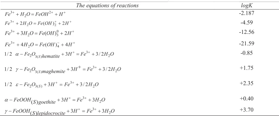
Table 1 The equilibrium constants of the analyzed reactions.

The equations of reactions _logK

  _{H OFeOH H}

Fe 3 2 2

-2.187

  _{ H OFe OH  H}

Fe 3 2 2 ( )2 2

-4.59 

_{ HOFe OH  H}

Fe 3 3 ₂ ( )₃0 2 -12.56

  _{ H OFe OH  H}

Fe 3 4 2 ( )4 4

-21.59 O H Fe H hematite O

Fe 2 3(_S) 3 3 3/2 2

2 /

1 _   

-0.85 O H F e H maghemite O

Fe 2 3(_S) 3 3 3/2 2

2 /

1 _   

+1.75 O H F e H O

Fe 2 3(S) 3 3 3/2 2

2 /

1 _   

+2.35 O H F e H goethite S

FeOOH ₃ 3 _{3 2}

) (        +0.40 O H F e H ite lepidocroc S

FeOOH_{( )} 3  3 3 ₂

  



+3.70

q y

The equations of reactions logK

HO FeOH H

Fe3 2 2 -2.187

_{H O FeOH H}

Fe3 2 2 ( )2 2 -4.59

_{H O FeOH H}

Fe 3 ( )0 2

3 2 3 _-12.56

H O FeOH H

Fe3 4 2 ( )4 4 -21.59

O H Fe H hematite O

Fe2 3(_S) 3 3 3/2 2

2 /

1 D -0.85

O H Fe H maghemite O

Fe2 3(_S) 3 3 3/2 2

2 /

1 J +1.75

O H Fe

H O

Fe2 3(S) 3 3 3/2 2

2 /

1 H +2.35

O H Fe H goethite S

FeOOH_{( )} 3 3 3 ₂

D +0.40 O H Fe H ite lepidocroc S

FeOOH ₃ 3 _{3 2}

)

(

Continuation of Table 1

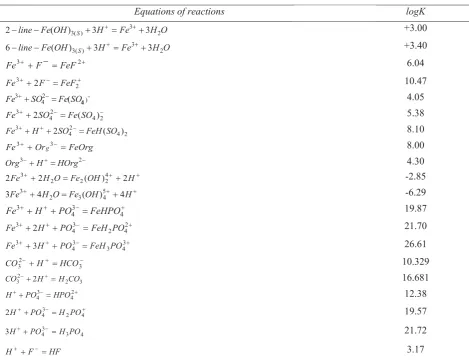
Equations of reactions _logK

O H F e H OH Fe

line ( )_3(S) 3 3 3 ₂

2     +3.00

O H F e H OH F e

line ( )_3(S) 3 3 3 ₂

6      +3.40

 _ _ 2

3 _{F FeF}

F e 6.04   _{ } 2 3 _{2F FeF}

F

e 10.47





 

 2 ₎

4 3 ₍ 4 SO Fe SO Fe 4.05   _{ } 2 4 2 4

3 _{2SO Fe (SO )}

F e 5.38 2 4 2 4

3 _{H 2SO FeH(SO )}

Fe    8.10

FeOrg O

r Fe 3 g3

8.00 



_{ } 2

3 _{H HOrg}

Org 4.30

  _{ H OFe OH  H}

Fe 2 ( ) 2

2 4 2 2 2 3 -2.85   _{ H OFe OH  H}

Fe 4 ( ) 4

3 5 4 3 2 3 -6.29    _{  } 4 3 4

3 _{H PO FeHPO}

F

e 19.87

 



_{  } 2

4 2 3

4

3 _{2H PO FeH PO}

F

e 21.70

 



_{  } 3

4 3 3

4

3 _{3H PO FeH PO}

F e 26.61   _{ } 3 2

3 H HCO

C

O 10.329

3 2 2

3 2H H CO

CO   16.681

 

_{ } 2

4 3 4 HPO PO H 12.38   _{ } 4 2 3 4

2H PO H PO 19.57

4 3 3 4

3HPO H PO 21.72

3.17 Figure 1 shows the calculation results of the buffer capacity S

Fe

E as a function of pH for the various iron (III) minerals. The analysis of the derived equations for the heterogeneous system showed that the increase in the total concentration 0

Fe

C for the pH values above 4.5, as well as the nature of the mineral have an insignifi cant effect on the area of the buffer action of studied system due to the very low solubility of iron oxy - hydroxides minerals. The appearance of maxima on the curves S

H

 (рН) and S Fe

E (рН) (Figures 1-3) is due to the dissociation process of carbonic acid with formation of HCO₃- _{ions (pH = 6.36) and CO}

32-(pH = 10.34).

2 3 4 5 6 7 8 9 10 11 12

0,0 1,0x10-4 2,0x10-4 3,0x10-4 7 6 5 3,4 2 1



_H

pH

C0_Fe = 1 x 10-4M Figure 1. The curves of dependence

of the buffer capacity β_H on pH for the system “Iron (III) mineral - saturated aqueous solution”. The

used concentrations (mol L-1_):

E ( ) 3 0 CO 4 0 SO 0 PO 0 Org 6 0 F 4 0 Fe 10 1 C , 10 1 C C C , 10 5 C , 10 1 C 3 4 4 ˜ ˜ ˜ ˜

1 - α-Fe₂O₃ (hematite), 2 - γ-Fe₂O₃ (maghemite), 3 – ε-Fe₂O₃,

4 - α-FeOOH (goethite), 5 - γ-FeOOH (lepidocrocite), 6 – Fe(OH)₃ (2-line ferrihydrite), 7 – Fe(OH)₃ (6-line ferrihydrite).

Equations of reactions logK

O H Fe H OH Fe

line ( )_3(S) 3 3 3 ₂

2 +3.00

O H Fe H OH Fe

line _S 3 ₂

) (

3 3 3

) (

6 +3.40

2

3 _{F FeF}

Fe 6.04

2

3 _{2F FeF}

Fe 10.47 2 ₎ 4 3 ₍ 4 SO Fe SO Fe 4.05 2 4 2 4

3 _{2SO Fe(SO )}

Fe 5.38

2 4 2

4

3 _{H 2SO FeH(SO )}

Fe 8.10

FeOrg Or

Fe3 g3 8.00

2

3 _{H HOrg}

Org 4.30

H O Fe OH H

Fe 2 ( ) 2

2 3 2 2 42 -2.85

_{H O Fe OH H}

Fe 4 ( ) 4

3 3 _{2 3} 5₄ -6.29

4 3 4

3 _{H PO FeHPO}

Fe 19.87 2 4 2 3 4

3 _{2H PO FeH PO}

Fe 21.70

43 3 43

3 _{3H PO FeH PO}

Fe 26.61 3 2

3 H HCO

CO 10.329

3 2 2

3 2H H CO

CO 16.681

2 4 3 4 HPO PO H 12.38 4 2 3 4

2H PO H PO 19.57

4 3 3 4

3HPO H PO 21.72

HF F

2 4 6 8 10 12 0,0

5,0x10-6

1,0x10-5

1,5x10-5

2,0x10-5

2,5x10-5

3,0x10-5

3,5x10-5

76 5 3,4 2 1

S Fe

pH

Figure 2. The curves of dependence of the buffer capacity S Fe

E on pH for the system “Iron (III) mineral - saturated aqueous solution”. The used concentrations (mol L-1_):

3 0

CO 4 0

SO 0

PO 0

Org 6 0

F 4 0

Fe 1 10 , C 5 10 , C C C 1 10 , C 1 10

C

3 4

4

_{˜ ˜ ˜}

˜ .

1 - α-Fe₂O₃ (hematite), 2 - γ-Fe₂O₃ (maghemite), 3 – ε-Fe₂O₃, 4 - α-FeOOH (goethite), 5 - γ-FeOOH (lepidocrocite), 6 – Fe(OH)₃ (2-line ferrihydrite), 7 - Fe(OH)₃ (6-line ferrihydrite).

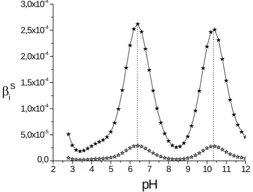
2 3 4 5 6 7 8 9 10 11 12

0,0 5,0x10-5

1,0x10-4 1,5x10-4 2,0x10-4

2,5x10-4

3,0x10-4



_iS

pH

Figure 3. Buffer capacities S H

 (1) and S Fe

E (2) versus pH for the system “Hematite - saturated aqueous solution”.

The used concentrations (mol L-1_): 0 3

CO 4 0

SO 0

PO 0

Org 6 0

F 5 0

Fe 1 10 , C 5 10 , C C C 1 10 , C 1 10

C _{˜ ˜ 4 4 ˜ 3 ˜ .}

The iron (III) ions and its complexes have a signifi cant contribution only in very acidic solutions up to pH 4.5. The analysis of the data presented in Figures 2 and 3 allows us to conclude that the studied heterogeneous system has a buffer capacity in relation to ions of hydrogen and iron (III). We will note down that these relations are valid only in the presence of solid phases.

Another example of real natural system that we examined is “Gibbsite – saturated aqueous solution”. By increasing the acidity in aqueous solutions the content of aluminium grows quickly due to the interaction of the gibbsit with an acid:

3 3

2 3 )

(

3 3 3 , [ ][ ]

)

(_{OH H Al H O K Al H}

Al _{S S}

An important interrelation between the buffer capacities of the heterogeneous system “Gibbsite Al(OH)_3(s) - saturated aqueous solution” system can be identifi ed [53,54]:

S Al S H E

Besides the process of gibbsite dissolution, a set of possible equilibria in the system “Mineral phase – natural water”, listed in Table 2 has been taken into account [52]. The following composition of the heterogeneous system has been used for the calculations: 0

Al

C = 1∙10-4 _{mol L}-1_, 0

F

C = 5∙10-6 _{mol L}-1_, 0

Org

C = 1∙10-4 _{mol L}-1_, 0

4

PO

C = 1∙10-4 _{mol L}-1_,

0

4 SO

C _{= 1∙10}-4 _{mol L}-1 _and 0

3 CO

C = 1∙10-3 _{mol L}-1_{. One can state that the infl uence of H}+ _{in the studied pH interval may be} neglected, and the OH– _{ions exercise infl uence on} S

H

 only at pH > 8.5. The aluminium ions and their hydroxocomplexes make a signifi cant contribution in acid solutions up to рН 5.5 and at рН > 8 because of the predominance of the stable anionic hydroxocomplex Al(OH)₄-_{. The results of the calculations of the buffer capacities} S

H

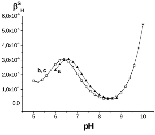
 as a function of рН for different compositions of the heterogeneous mixture are shown in Figures 4–5. Obviously, an increase of the total concentration 0

Al

C (Figure 4) augments the area of the buffer action because of the extension of the рН interval of the

thermodynamic stability of the solid phase. At concentrations of fl uoride 0 F

C = 5∙10-4 _{mol L}-1_{, the} S

H

 value increases sharply in the range of pH values of the gibbsite dissolution – formation with a simultaneous narrowing of the total pH range of the buffer action (Figure 5).

Table 2 Equilibrium constants and values of enthalpies (ΔH).

Equations of reactions log K ΔH (cаl mоl–1₎

  _{H O AlOH H}

Al 2

2

3 -4.99 11900

  _{ HOAl OH  H} Al3 2 2 ( )2 2

-10.00 22000

  _{ H OAl OH  H}

Al3 4 2 ( )4 4

-23.00 44060 O H A l H O H

Al( )3(S)3   33 2

9.35 –22800

 

_{ } 2

3 _{F AlF}

A l 7.02 1100   _{ } 2 3 _{2F AlF}

Al 12.76 2000

3 3 _{3F AlF}

Al    17.03 2500

 

_{ }

4 3 _{4F AlF}

A

l 19.73 2200

 

_{ } 2

5 3 _{5F AlF}

Al 20.92 1800

   _{ } 4 2 4

3 _{SO AlSO}

A

l 3.01 2150

  _{ } 2 4 2 4

3 _{2SO Al (SO )}

A

l 4.90 2840

AlOrg Org

Al3 3 8.39 —

 



_{H Org AlHOrg}

Al3 3 13.09 —

 

_{ } 2

3 _{H HOrg}

Org 6.83 —

 

_{ H H Org}

Org3 2 ₂ 12.73 —

Org H H

Org33  ₃ 14.49 —

HF F

H  3.17 3460

 _ H OH O

H2

-14.00 13340

  _{ H OAl OH  H}

Al 2 ( ) 2

2 4

2 2 2

3 -6.3 —

   _{ H OAl OH  H}

Al 4 ( ) 4

3 3 _{2 3} 5₄ -12.1 —

 

_{ } 2 4 2 4 2

3 _{H PO AlH PO}

A

l 3.1 —

 

_{ } 2 4 3

4 H HPO

P

O 12.0 —

 _ _

4 2 3

4 2 H PO

PO H

19.21 —

4 3 3

4 3H H PO

PO   21.36 —

Note: 1 cal = 4.184 J, Org - organic ligand, the „—” specifi es the absence of experimental data.

Equations of reactions log K ǻH (cɚl mɨl–1

)

_{H O AlOH H}

Al3 ₂ 2 -4.99 11900

HO AlOH H

Al3 2 2 ( )2 2 -10.00 22000

H O Al OH H

Al3 4 2 ( )4 4 -23.00 44060

O H Al H OH

Al( )3(S)3 33 2 9.35 –22800

2 3 AlF F

Al 7.02 1100

2

3 _{2F AlF}

Al 12.76 2000

3 3 ₃

AlF F

Al 17.03 2500

4

3 _{4F AlF}

Al 19.73 2200

2 5 3 ₅ AlF F

Al 20.92 1800

4 2 4

3 _{SO AlSO}

Al 3.01 2150

42 4 2

3 _{2 ( )}

SO Al SO

Al 4.90 2840

AlOrg Org

Al3 3 8.39 —

_{H Org AlHOrg}

Al3 3 13.09 —

2 3 HOrg H

Org 6.83 —

_{H H Org}

Org3 2 ₂ 12.73 —

Org H H

Org33 ₃ 14.49 —

HF F

H 3.17 3460

OH

H O

H2 -14.00 13340

_{HO Al OH H}

Al 2 ( ) 2

2 3 _{2 2} 4₂ -6.3 —

_{H O Al OH H}

Al 4 ( ) 4

3 5

4 3 2

3 _{-12.1 —}

2 4 2 4 2

3 _{H PO AlH PO}

Al 3.1 —

2

4 3

4 H HPO

PO 12.0 —

4 2 3

4 2 H PO

PO H 19.21 —

4 3 3

4 3H H PO

PO 21.36 —

Note: 1 cal = 4.184 J, Org - organic ligand, the „—” specifies the absence of experimental data.

5 6 7 8 9 10 0,0

1,0x10-4

2,0x10-4

3,0x10-4 4,0x10-4 5,0x10-4 6,0x10-4



S

H

b, c a

pH

Figure 4. Buffer capacity S H

 versus pH for the “Gibbsite - saturated aqueous solution” system. Concentrations (mol L-1_):

3 0

C O 4 0

SO 0 PO 0 Org 6 0

F -5 4

3 0

Al :a 1 10 ,b 1 10 ,c-1 10 , C 5 10 , C C C 1 10 , C 1 10

C _{ }  _{ }  _{  }  _{ 4  4  }  _{3  } 

.

4 5 6 7 8 9 10

0,0 1,0x10-4 2,0x10-4

3,0x10-4 4,0x10-4

5,0x10-4



S

H

1 3 1, 2 4

pH

Figure 5. Buffer capacity S H

 versus pH for the “Gibbsite - saturated aqueous solution” system. Concentrations (mol L-1_):

3 0

C O 4 0

SO 0 P O 0 Org 0

A l -4 -5

6 7

0

F:1 5 10 ,2 5 10 ,3-5 10 ,4 -5 10 C C C C 1 10 , C 1 10

C _{ }  _{ }  _{  ,   4  4  }  _{3  } 

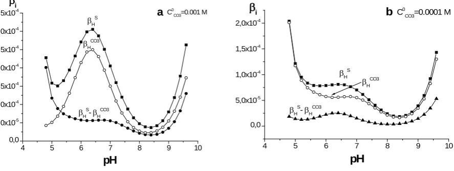
The dependences of HS(рН) for different concentrations of carbonate ion are presented in Figure 6. By taking into account the contribution of equilibria including carbonate ion in the total buffer capacity S

H

 , the ECOH₃value

was calculated separately. A comparison of the calculated curves shows that equilibria with CO₃2- _{participation have} a substantial contribution to S

H

 at a 0 ₁₁₀4

3 ˜ !

CO

C mol L-1 _{(Figures 7а and 7b). The analysis of the obtained data}

. Figure 4. Buffer capacity S

H

E versus pH for the “Gibbsite - saturated aqueous solution” system. Concentrations (mol L-1_):

3 0

CO 4 0

SO 0

PO 0

Org 6 0

F -5 4

3 0

Al:a 1 10 , b 1 10 , c-1 10 , C 5 10 , C C C 1 10 , C 1 10

C _{˜ ˜ ˜ ˜ 4 4 ˜ 3 ˜}

Figure 5. Buffer capacity S H

E versus pH for the “Gibbsite - saturated aqueous solution” system. Concentrations (mol L-1):

3 0

CO 4 0

SO 0

PO 0

Org 0 Al -4 -5

6 7

0

F:1 5 10 , 2 5 10 , 3-5 10 , 4-5 10 C C C C 1 10 , C 1 10

C _{4 4 3}

˜ ˜

˜ ˜

˜ ˜

,

.

presented in Figures 4–7, taking into account Eq.(33) allows us to conclude that the investigated heterogeneous system has a considerable buffer capacity towards to aluminium as well.

5 6 7 8 9 10

0,0 5,0x10-4 1,0x10-3 1,5x10-3 2,0x10-3 2,5x10-3 3,0x10-3

S H

3 2 1

pH

Figure 6. Buffer capacity S H

 versus pH for the “Gibbsite - saturated aqueous solution” system. Concentrations (mol L-1_):

6 0

F 4 0

SO 0 P O 0 A l -4 3

2 0

CO :1 1 10 ,2 1 10 ,3-1 10 C C C 1 10 , C 5 10

C

4 4 3

 



 _{        }



 ,

4 5 6 7 8 9 10

0,0 5,0x10-5 1,0x10-4 1,5x10-4 2,0x10-4 2,5x10-4 3,0x10-4

3,5x10-4 _a

_i

C0 CO3=0.001 M

_HS

- _HCO3

_HCO3

_HS

pH

4 5 6 7 8 9 10

0,0 5,0x10-5 1,0x10-4 1,5x10-4 2,0x10-4

_{i bC}0

CO3=0.0001 M

_HS

- _HCO3

_HCO3

_HS

pH

Figure 7. Total buffer capacity S H

 versus pH, carbonate buffer capacity



COH₃ vs. pH and their difference S

H

 – _COH₃ for the “Gibbsite - saturated aqueous solution” system.

Concentrations (mol L-1_): 0 6

F 4 0

SO 0 PO 0 A l -4 3

0

CO :a 1 10 ,b-1 10 C C C 1 10 , C 5 10

C ₃     ,  ₄  ₄      

The infl uence of temperature on the value of the buffer capacity was also studied [55]. The results of the calculations are presented in Figure 8. The equilibrium constants for different temperatures have been estimated by the Van’t Hoff equation.

logK₂ = logK₁ + (1/T₁ – 1/T₂) ΔH/2.303R

The necessary values of enthalpies (ΔH) are listed in Table 2. T₁ was set to 298 K = 25 °C. It was assumed that the temperature insignifi cantly infl uences the ΔH values inside the investigated temperature range. An analysis of the curves in Figure 8 shows that the buffer capacity increases with a temperature decrease, whereas the рН interval of 5.5 – 7.0 of the maximum values of the buffer capacity displaces slightly.

Figure 6. Buffer capacity S H

E versus pH for the “Gibbsite - saturated aqueous solution” system. Concentrations (mol L-1_):

6 0

F 4 0

SO 0

PO 0 Al -4 3

2 0

CO :1 1 10 , 2 1 10 , 3-1 10 C C C 1 10 , C 5 10 C

4 4 3

˜ ˜

˜ ˜

˜

,

Figure 7. Total buffer capacity S H

E versus pH, carbonate buffer capacity

E

COH₃ vs. pH and their difference

S H

E – H

CO3

E for the “Gibbsite - saturated aqueous solution” system.

Concentrations (mol L-1_): 0 6

F 4 0

SO 0

PO 0 Al -4 3

0

CO : a 1 10 , b-1 10 C C C 1 10 , C 5 10

C _{3 4 4}

˜ ˜

˜ ˜

,

Concentrations (mol L-1_): 0 6

F 4 0

SO 0

PO 0 Al -4 3

0

CO : a 1 10 , b-1 10 C C C 1 10 , C 5 10

C _{3 4 4}

˜ ˜

˜ ˜

,

.

4 5 6 7 8 9 10 0,0

1,0x10-4

2,0x10-4

3,0x10-4

4,0x10-4



_HS

4 3 2

1

pH

Figure 8. Buffer capacity



_HS versus pH for the “Gibbsite - saturated aqueous solution” system at different temperatures (t, °С): (1) –5, (2) +10, (3) +25 and (4) +40.

Concentrations (mol L-1_): 0 6

F 4 0

SO 0

P O 0 A l 3 0

CO 1 10 ,C C C 1 10 , C 5 10

C

4 4

3

 

 _{      }



 0

Org C

Buffer properties for liquid two-phase acid-base buffer systems

Buffer with mono- and diprotic acids

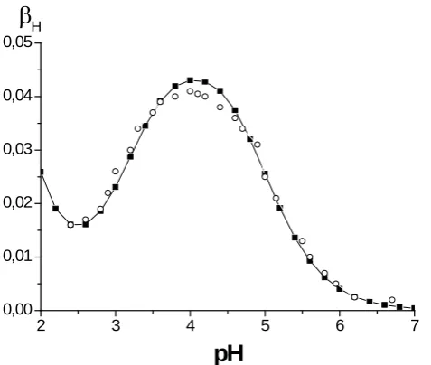
The theoretically calculated and experimentally measured dependences of the buffer capacity on pH in the case of two-phase system 1-octanol – water for monoprotic n-hexanoic acid and diprotic 1,2-benzenedicarboxylic acid are shown in Figure 9 and Figure 10, respectively. Experimental data [45,56] were obtained at 25 0_{C and constant ionic}

strength. For both systems, the experimental data correlate well with the theoretical curves, calculated by Eqs.(27 – 28) that confi rms their correctness. The values in Figures 9 and 10 testify the validity of Eq.(29). (The necessary equilibrium constants were taken from [45,56].)

5,0 5,5 6,0 6,5 7,0 7,5 8,0 8,5 9,0 0,00

0,01 0,02 0,03 0,04 0,05 0,06



H

, m

o

l/L

pH

Figure 9. Buffer capacity versusрН for two-phase system containing n-hexanoic acid HA and 1-octanol: (■) the calculated values; (◊) experimental data [56];

1-octanol : water = 1:1; 0

A

C = 0.1 mol L-1_{, I = 0,t = 25} 0_C.

Figure 8. Buffer capacity

E

_HS versus pH for the “Gibbsite - saturated aqueous solution” system at different temperatures (t, °ɋ): (1) –5, (2) +10, (3) +25 and (4) +40.

Concentrations (mol L-1): 0 6

F 4 0

SO 0

PO 0 Al 3 0

CO 1 10 ,C C C 1 10 , C 5 10

C

4 4

3

_{˜ ˜}

2 3 4 5 6 7 0,00

0,01 0,02 0,03 0,04 0,05



_H

pH

Figure 10. Dependence of buffer capacity on рН for two-phase system containing 1,2-benzenedicarboxylic acid and 1-octanol: (■) calculated values; (○) experimental data [45];

1-octanol : water=1:1; 0 A

C = 0.0488 mol L-1_{, I = 1 (NaCl), t = 25} 0_C.

Two-phase buffers with monoprotic acids in which dimerization occurs

Mono-component systems: propanoic acid – water – benzene (I) and decanoic acid – water – benzene (II): The numerical values of the equilibrium constants used for calculating the theoretical buffer curves as well as the experimental data were taken from [56]. The theoretical and experimental data are presented in Figure 11 (a,b). It can be seen that the theoretical curves are in good agreement with experimental values.

a

3 4 5 6 7 8 9 10 0,000

0,005 0,010 0,015 0,020 0,025 0,030 0,035

0,040 2

1

_

pH

b

3 4 5 6 7 8 9 10

0,00 0,01 0,02 0,03 0,04 0,05 0,06 0,07

0,08 2

1

_

pH

Figure 11. Buffer capacity β_H versus pH for mono-component two-phase systems with propanoic (a) and decanoic (b) acids, 0

A

C =0.05 mol L-1 _{(a) and} 0

A

C =0.1 mol L-1 _{(b) and α = 1;}

(■) – experimental values, dotted lines – experimental curves, I = 0.1, t = 25 0_C.

3,0 3,5 4,0 4,5 5,0 5,5 6,0 6,5 7,0 0,00

2,50x10-3

5,00x10-3

7,50x10-3

1,00x10-2 1,25x10-2 1,50x10-2

5 4 3 2

1



_H

pH

Figure 12. Buffer capacity β_H versus pH for mono-component two-phase systems with (2.4-dichlorophenoxy) acetic acid, 0

A

C = 0.05 mol L-1_{, α = 1, t = 25} 0_{C for different organic solvents:}

1 – no solvent; 2 – ethylbenzene; 3 – 1-octanol; 4 – chlorbenzene; 5 – nitrobenzene.

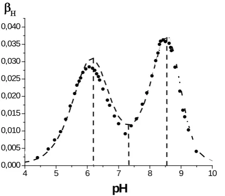
pH and pA buffer properties of two-component system in which mixed dimmer occurs

The authors [56] found that the rule of additivity for calculating the total buffer capacity as a sum of separate contributions for this system is not valid. As a result, there are some substantial deviations of the theoretical curves from experimental data within the interval of pH from 4 to 7. The experimental data for this system, along with the calculated theoretical curve are presented in Figure 13. As one can see, the experimental values β_H = f(pH) are in good agreement with those calculated, contrasting to the results received by authors [56]. Thus, the experiment confi rms the validity of our developed theoretical approach.

4 5 6 7 8 9 10

0,000 0,005 0,010 0,015 0,020 0,025 0,030 0,035 0,040



_

pH

Figure 13. Experimental data [56] (

•

) and calculated values (---) for β_H(pH) as a sum of the contributions of separate acids for the two-component two-phase buffer system containing hexanoic and decanoic acids.



CH

 

VHO



1 1

V 6 6  2   , C0ACB00.05 mol L-1, I = 0.1, t = 25 0C.

4 5 6 7 8 9 10 0,00

0,02 0,04 0,06 0,08 0,10 0,12

_ _

_



_i

pH

Figure 14. Curves β_H = f(pH),β_А = f(pH) and β_B = f(pH) for the two-component two-phase buffer system, containing hexanoic and decanoic acids. V



C₆H₆

 

V H₂O



11, 0 0 

B A C

C 0.05 mol L-1_{, I = 0.1, t = 25} 0_C.

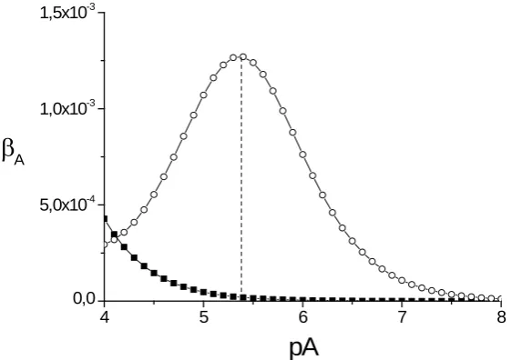
On Figure15 the functional dependence β_A = f(pA) for (2.4-dichlorophenoxy)acetic acid for aqueous solution and water-1-octanol mixture is depicted. One can notice that the presence of organic solvent amplifi es signifi cantly (approximately by 70 times) the β_A value at pA = 5.4. Therefore, two-phase mixtures can be successfully used for designing new buffers with respect to any component for investigated systems. The developed approach can be expanded to other, more complicated systems, containing metal-ligand complexes.

4 5 6 7 8

0,0 5,0x10-4

1,0x10-3

1,5x10-3



_A

pA

Figure 15. Buffer capacity β_A versus pA for the mono-component system with (2.4-dichlorophenoxy) acetic acid in water (curve 1) and water-1-octanol mixture (curve 2), 0

H

C =0.005 mol L-1_{, α = 1; t = 25} 0_C.

Conclusions