A NEW APPROACH TO SELF-LOCALIZATION FOR
MOBILE ROBOTS USING SENSOR DATA FUSION
B. Moshiri
Department of Electrical and Computer Engineering, Faculty of Engineering University of Tehran, P.O.Box: 14395/515, Tehran, Iran, [email protected]
M. R. Asharif
Department of Information Engineering, Faculty of Engineering University of Ryukyus, Okinawa, Japan, [email protected]
R. HoseinNezhad
Department of Electrical and Computer Engineering, Faculty of Engineering University of Tehran, P.O.Box: 14395/515, Tehran, Iran, [email protected]
(Received: July 5, 2001 – Accepted: October 23, 2001)
Abstract This paper proposes a new approach for calibration of dead reckoning process. Using the well-known UMBmark (University of Michigan Benchmark) is not sufficient for a desirable calibration of dead reckoning. Besides, existing calibration methods usually require explicit measurement of actual motion of the robot. Some recent methods use the smart encoder trailer or long range finder sensors such as ultrasonic or laser range finders for automatic calibration. Manual measurement is necessary in the case of the robots that are not equipped with long-range detectors or such smart encoder trailer. Our proposed approach uses an environment map that is created by fusion of proximity data, in order to calibrate the odometry error automatically. In the new approach, the systematic part of the error is adaptively estimated and compensated by an efficient and incremental maximum likelihood algorithm. Actually, environment map data are fused with the odometry and current sensory data in order to acquire the maximum likelihood estimation. The advantages of the proposed approach are demonstrated in some experiments with Khepera robot. It is shown that the amount of pose estimation error is reduced by a percentage of more than 80%.
Key Words Sensor Data Fusion, Pose Estimation, Dead Reckoning Calibration, Occupancy Grids, Maximum Likelihood, Map Building
ﻩﺪﻴﻜﭼ
ﻩﺪﻴﻜﭼ
ﻩﺪﻴﻜﭼ
ﻩﺪﻴﻜﭼ
ﺭﺩ
ﺪﻨﻳﺍﺮﻓﺭﺩﺩﻮﺟﻮﻣﻱﺎﻄﺧﻥﺩﺮﻛﻩﺮﺒﻴﻟﺎﻛﻱﺍﺮﺑﻱﺪﻳﺪﺟﺵﻭﺭﻪﻟﺎﻘﻣﻦﻳﺍ DEAD RECKONING
ﺕﺎﺑﺭﻲﺑﺎﻳﻥﺎﻜﻣﺩﻮﺧﻱﺍﺮﺑ
ﺖﺳﺍﻩﺪﺷﺩﺎﻬﻨﺸﻴﭘﻙﺮﺤﺘﻣ .
ﻪﻠﺻﺎﻓﻱﺎﻫﺭﻮﺴﻨﺳﺕﺎﻋﻼﻃﺍﺐﻴﻛﺮﺗﺯﺍﻪﻛﻂﻴﺤﻣﺖﺷﺎﮕﻧﻚﻳﺯﺍﺵﻭﺭﻦﻳﺍﺭﺩ ﻩﺪﺷﻞﺻﺎﺣﺞﻨﺳ
ﺩﻮﺷﻲﻣ ﻩﺩﺎﻔﺘﺳﺍﻚﻴﺗﺎﻣﻮﺗﺍ ﻥﻮﻴﺳﺍﺮﺒﻴﻟﺎﻛﻦﻳﺍ ﻡﺎﺠﻧﺍﻱﺍﺮﺑ ،ﺖﺳﺍ .
ﻲﻘﻴﺒﻄﺗ ﻲﻠﻜﺸﺑﻱﺮﺘﻣﻭﺩﺍﻱﺎﻄﺧ ﻚﻴﺗﺎﻤﺘﺴﻴﺳ ﺶﺨﺑﻊﻗﺍﻭ ﺭﺩ
ﺖﻫﺎﺒﺷﺮﺜﻛﺍﺪﺣﺮﮕﻨﻴﻤﺨﺗﻚﻳﺎﺑﻩﺪﺷﻩﺩﺯﻦﻴﻤﺨﺗ ،
ﻲﻣﻱﺯﺎﺳﻥﺍﺮﺒﺟ ﺩﺩﺮﮔ
. ﺍﺭﻩﺪﺷﻪﺒﺳﺎﺤﻣﻥﺎﻜﻣ،ﻥﻮﻴﺳﺍﺮﺒﻴﻟﺎﻛﻦﻳﺍﻦﻴﺣ ﺭﺩ
ﻋﻼﻃﺍﺐﻴﻛﺮﺗﻪﺠﻴﺘﻧﻥﺍﻮﻨﻌﺑﻥﺍﻮﺗﻲﻣ
ﺩﻮﻤﻧﺏﻮﺴﺤﻣﺏﺎﻳﻪﻠﺻﺎﻓﻱﺎﻫﺭﻮﺴﻨﺳﺕﺎﻋﻼﻃﺍﻭﻱﺮﺘﻣﻭﺩﺍﺕﺎ .
ﻥﻮﻴﺳﺍﺮﺒﻴﻟﺎﻛﻦﻳﺍﻱﺎﻳﺍﺰﻣ
ﻙﺮﺤﺘﻣ ﺕﺎﺑﺭﺎﺑ ﻩﺪﺷ ﻡﺎﺠﻧﺍﺶﻳﺎﻣﺯﺁ ﻭﺩﺭﺩ ﻚﻴﺗﺎﻣﻮﺗﺍ KHEPERA
ﺪﻧﺍﻩﺪﺷ ﻩﺩﺍﺩﻥﺎﺸﻧ ﻲﺑﻮﺨﺑ .
ﻥﺍﺰﻴﻣﻪﻛ ﺩﺩﺮﮔﻲﻣ ﻩﺪﻫﺎﺸﻣ
،ﺕﺎﺑﺭﺖﻴﻌﻗﻮﻣﻦﻴﻤﺨﺗﻱﺎﻄﺧ ﭘ
ﺯﺍﺶﻴﺑﻱﺩﺎﻬﻨﺸﻴﭘﺵﻭﺭﻱﺮﻴﮔﺭﺎﻜﺑﺯﺍﺲ ﺪﺻﺭﺩﺩﺎﺘﺸﻫ
ﻲﻣﺶﻫﺎﻛ ﺪﺑﺎﻳ .
1. INTRODUCTION
Almost, sufficient knowledge about the robot's pose (consisting of its position and the direction angle of its motion) is essential in every mobile robotic application. Usually the wheels of the robot are equipped with some motion encoders and a
significant systematic errors into the robot's odometry. The requirement for such calibration is as old as the field of robotics itself and the literature of methods for calibrating robots (for example see [1-5]). Well-nigh, all of the exiting calibration methods have certain disadvantages. Many existing calibration methods call for human intercession i.e. in order to calibrate a mobile robot's odometry, a person (or some external agent or device) has to measure the exact position and direction angle of the robot, and deduce the physical model from these measurements. Because of two reasons, such approaches are unsuitable. Firstly a considerable amount of endeavor is involved in calibration process of the robot that normally cuts it off from its continuous operation. Secondly and more importantly, the physical characteristics of the mobile robot and the environment around it changes. For robot arms, robotic platforms and many other stationary devices, the environment is mainly static. In addition, the odometry error of the robot arm joint is strictly internal to the joint and is not deviated due to most changes of the environment. On the other side, a mobile robot's odometry depends on the kind of surface that the robot is traveling on it. If the surface varies (e.g. from carpet to tile), then the calibration parameters change. Therefore, calibration process for such a robot, must be adaptive and in addition to pose estimation by dead-reckoning, mobile robot must fuse odometry data with a feedback from the environment. Normally, such a feedback is generated by sensory data. Existence of a rich chronicle of using multi sensor data fusion methods in mobile robotic applications (see [6,7,8,9] as some examples) enthuses us to fuse the sensory data with odometry data in order to compensate the errors and predict parameter variations. In such a localization process, robot's pose is estimated by utilizing both uncalibrated odometry and sensory data e.g. from a laser range finder sensor. Thus, the demand for a model of the odometry error is extinguished [10]. Thrun, has done a wide research in this area [11,12]. In his recent work [5], he implemented his algorithm on a mobile robot, that was equipped with long range finder sensors. He used a mathematical sensor model in his algorithm, that was based on ray tracing. In this method, the likelihood of a ``hit" depends on the occupancy probability of the grid cell that is being traced [13].
In our map building and navigation experiments, we used a simple Khepera robot. This robot is equipped only with infra-red proximity detectors [14]. The data, provided with such sensors, are appropriate for short distances only. Besides, there is no exact model to convert the proximity values to distance values and applying the ray tracing approach. In this paper, a new approach is introduced for compensation of the systematic part of the error that exists in odometry data. In our approach, a new maximum likelihood method is applied to estimate the parameters. In the process of approximating the likelihood ratio, the local maps that are extracted from a previously created global map, are compared with the local map that is developed by the current values of the infra-red sensors of the robot. Actually, the extracted local map, depends on both the global map data and the estimation of the robot's pose. Thus, corresponding to each dead reckoning parameter values, there is a different extracted map. In our method, we seek for the parameter values, corresponding to an extracted local map, that is best fitted with the local map, generated from current sensory data.
In the second section, probabilistic formulation of pose estimation by dead reckoning (using odometry data) is briefly reviewed. Then, the new method for maximum likelihood estimation, is introduced in the third section. Experimental results will be given in the fourth section. Finally, we will give conclusions in the last section.
2. ODOMETRY PARAMETERS: A BRIEF REVIEW
Robot motion is probabilistically modeled in our calibration method. More distinctly, let
T
)
,
y
,
x
(
θ
=
π
denotes the robot's pose in a two dimensional space (θ
is the robot's heading direction). Robot motion is modeled by the conditional probability distributionP
(
π
|'
π
,
d
)
whereπ
is the robot's pose before executing an action, d is the displacement measured by the robot's odometry, andπ
'
is the pose after executing the action. Assume thatd
trans(
k
)
and)
k
(
)
k
(
D
trans andD
rot(
k
)
are their real values respectively. If |l| is the distance, traveled between the two iterations, then our probabilistic model will be expressed as below:rot rot rot rot trans trans trans trans
e
|
l
|
)
k
(
d
)
k
(
D
e
|
l
|
)
k
(
d
)
k
(
D
+
×
α
+
=
+
×
α
+
=
(1)where the terms
α
trans(
k
)
×
|
l
|
andα
rot(
k
)
×
|
l
|
stand for the systematic error ande
trans ande
rot are zero-mean random variables and stand for the non-systematic error (refer to [3] for more details on systematic and non-systematic errors of odometry data). Calibration of the robot's pose estimation is defined by estimatingα
trans andα
rot.As (1) indicates, our model presumes that both errors increase linearly with the distance
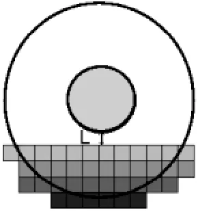
Figure 1. Robot’s kinematics, based on the values of
rotational and translational displacements, estimated by dead reckoning.
traveled. In practice, it has been found that this model is superior over other various choices, including models with more parameters [5]. Figure 1 shows a typical robot's kinematics. As it is demonstrated in the figure, robot's pose state transition can be expressed by the following equation: + θ × + = + + θ × + = + + θ = + θ )) k ( D ) k ( sin( ) k ( D ) k ( y ) 1 k ( y )) k ( D ) k ( cos( ) k ( D ) k ( x ) 1 k ( x ) k ( D ) k ( ) 1 k ( rot trans rot trans rot (2)
3. PARAMETER ESTIMATION
We estimate the parameters
α
trans andα
rot by using the sensory data and odometry data that have been gathered during robot motion, gradually. Actually, it is a maximum likelihood estimation problem and we search for the parameters that appear most plausible under the existing sensory and odometry data. This estimation is formulated as below:)
S
,
Q
|
,
(
P
max
arg
)
,
(
trans rot k k 1, T * rot * trans rot trans + α
α
α
α
=
α
α
(3) where Sk+1 means the sensory data (e.g. infra-red proximity or laser or ultrasonic range finder sensors or any other source of information related to environment perception) in the kth iteration and
k
Q
is the collection of the whole odometry and sensory information that is gathered in kthiteration or was stored before. More specifically, it can be defined by:
{
1 1 2 2 k k}
k
S
,
O
,
S
,
O
,
,
S
,
O
Q
=
L
where
O
i is the odometry data that is/was gathered ini
th iteration i.e. the erroneous measured values of translational and rotational displacements)
i
(
d
trans andd
rot(
i
)
.algorithm simpler and adaptive. In order to consider the variations of parameters and contribute adaptation to the estimation algorithm, a local maximum likelihood estimator as below estimates parameter values in each iteration:
) S , Q | , ( P max arg ) ,
( trans rot i i1
, T ) i *( rot ) i *( trans rot trans + α
α α α
= α
α (4)
and then, they are adapted by the following rule:
T * rot * trans T ) i *( rot ) i *( trans T * rot * trans ) , ( ) , ( ) 1 ( ) , ( α α → α α × γ − + α α × γ (5)
Here γ≤1 is an exponential forgetting factor, which decays the weight of measurements over time. It is usually selected near to 1 and was 0.9 in our experiments.
4. LIKELIHOOD FUNCTION
The only thing that is remained to be computed or approximated is the parameter likelihood function
)
S
,
Q
|
,
(
P
α
transα
rot i i+1 in (4). According to Bayesian rule, this value can be expressed as follows:)
Q
|
,
(
P
)
,
,
Q
|
S
(
P
)
S
,
Q
|
,
(
P
i rot trans rot trans i 1 i 1 i i rot transα
α
×
α
α
×
ς
=
α
α
+ + (6)where
ς
=
P
(
S
i+1|
Q
i)
−1 is a normalizing factor and can be ignored during the maximization process. The knowledge inO
i without knowing aboutS
i+1, contains no information related toα
*(transi) andα
*(roti). SoP
(
α
trans,
α
rot|
Q
i)
=
P
(
α
trans,
α
rot)
and this is a priori probability that may also be discarded while maximization. It remains to calculate or approximate the termP
(
S
i+1|
Q
i,
α
trans,
α
rot)
. We call this term sensation likelihood.5. ESTIMATION OF THE SENSATION LIKELIHOOD
Assume that W is the world and
∆
π
is the relativedisplacement between the robot's poses
π
i+1 andi
π
. According to the theorem of total probability, sensation likelihood can be calculated by:
π
∆
α
α
π
∆
×
α
α
π
∆
=
α
α
+ +∫∫
d
dW
)
,
,
Q
|
,
W
(
P
)
,
,
Q
,
,
W
|
S
(
P
)
,
,
Q
|
S
(
P
rot trans i rot trans i 1 i rot trans i 1 i (7)Since the sensor data
S
i+1 is independent fromQ
iand
α
trans,α
rot and the world W and the displacement data∆
π
are independent from each other, (7) can be expressed by:π
∆
α
α
π
∆
×
α
α
×
π
∆
=
α
α
+ +∫∫
d
dW
)
,
,
Q
|
(
P
)
,
,
Q
|
W
(
P
)
,
W
|
S
(
P
)
,
,
Q
|
S
(
P
rot trans i rot trans i 1 i rot trans i 1 i (8)Besides, we know that W is independent of the motion data and parameters. Also
∆
π
depends only on the recent motion dataO
i and theα
parameters. Thus (8) can be more simplified as follows:π
∆
α
α
π
∆
×
×
π
∆
=
α
α
+ +∫∫
d
dW
)
,
,
Q
|
(
P
)
S
,...,
S
,
S
|
W
(
P
)
,
W
|
S
(
P
)
,
,
Q
|
S
(
P
rot trans i i 2 1 1 i rot trans i 1 i (9)Of course, integrating over all possible worlds W and all displacements
∆
π
is infeasible. We can approximate the sensation likelihood by substituting the integrals in (9) with their expected values. They are much easier to calculate. Finally the following expression, is proposed as a close approximation for the sensation likelihood:[
]
(
[
i trans rot]
)
where E[.] is an indication of the conditional expected quantity of a random variable.
6. CALCULATION OF THE EXPECTATIONS AND THE APPROXIMATED LIKELIHOOD
In this subsection, it is explained that how the two expected values and the approximated likelihood in (10) are calculated in our approach. The first term, E
[
W |S1,S2,...,Si]
is considered as a global occupancy grids map of the environment, that has been generated up to the thi iteration. There is a large set of methods for creation of such a map. It can be generated by Bayesian fusion of sensory data [15,16] or by a more intelligent neural-Bayesian approach [9] or by our new method, called pseudo information fusion [17,18]. Although there are several approaches for environment mapping in mobile robotics, occupancy grids has been selected (See [11] for more information about mapping methods and map learning). That is because a grid-based map can be easily created, handled and applied to the likelihood estimation, as it will be shown later in this subsection. T he second expectation term
[
|
Q
i,
trans,
rot]
E
∆
π
α
α
is an expected displacement vector, denoted by[
i trans rot]
T
,
,
Q
|
)
,
y
,
x
(
E
∆
∆
∆
θ
α
α
where
O
i=
(
d
trans,
d
rot,
|
l
|)
T is the recent movement information that is obtained by using the wheel encoders data. Equations 1 and 2 can be utilized to calculate the expected value of∆
π
, knowing the above information. But the non-systematic error term in (1) must be ignored because there exist no information about its value.The final term that is remained to be calculated is the sensation likelihood itself, i.e.
)
,
W
|
S
(
P
i+1∆
π
. This is the likelihood of the scan, recorded in the final position. If the sensors are long distance range finders (e.g. laser or ultrasonic sensors), then the likelihood value may be obtained by a simple ray tracing. In that case, the likelihood of a “hit” depends on the occupancy of the grid cell that is beingtraced. Consequently, sensor measurements that are more fitted to the occupancy grids map will get a higher likelihood value, while measurements that contradict the map, will be assigned a lower likelihood. See [5,13] for more details.
If the robot is not equipped with long range finder sensors, but only with some proximity range detectors (e.g. infra-red proximity detectors in the case of a Khepera miniature robot), then ray tracing cannot be applied to the likelihood estimation problem. In such a case, we may use the idea of local map matching. It is based on the fact that any sensor scan is uniquely corresponded to a local map around the robot. More specifically, there is a transformation T that transforms a sensor scan
1 +
i
S
to a local mapΓ
, i.e.Γ
=
Τ
(
S
i+1)
. In our experiments with Khepera, this transformation has been implemented by using a feed forward neural network (multi-layered perceptron). We will discuss it in the next section. It is assumed that this transformation is a one-to-one correspondence (i.e. two different sensor measurements are transformed to two different local maps around the robot). This assumption is practically valid. So, the sensation likelihood may be expressed as below:)
,
W
|
(
P
K
)
,
W
|
S
(
P
i+1∆
π
=
×
Γ
∆
π
(11)where K is a factor that can be ignored during maximization. Knowing a global map of the environment (or the world model W) and an estimated location of the robot in this map (calculated by the information in
∆
π
), one can easily extract a previously known local map around the robot calledΓ
'
. We interpret the conditional probabilityP
(
Γ
|
W
,
∆
π
)
as a judgment about the existing fitness between these two local maps. This fitness is formulated by the following equation:2
/
I
'
2
/
I
'
1
)
'
,
(
f
−
Γ
+
−
Γ
Γ
−
Γ
−
=
Γ
Γ
(12)norm, defined by:
∑∑
=
i j ij
a
A
||
|
|
||
(13)This fitness measure is normalized to [0,1] interval. In an ideal case, where
Γ
andΓ
'
are absolutely matched, this factor becomes 1. In the worst case, where the two maps are contradicting completely i.e.γ
ij+
γ
'
ij=
1
the fraction part of the expression will have a numerator equal to its denominator and so, this factor will be zero.Actually, only if there is sufficient occupied area around the robot, then (12) is a valid measure for the fitness between the two local maps. A threshold,
µ
min, is introduced for the total existing occupancy in both of the local maps. Parameter calibration by maximum likelihood will take place if the following occupancy condition is true:min
'
≥
µ
Γ
+
Γ
(14)As a simple example, two typical local maps around the robot are shown in Figures 2 and 3. They have been extracted from a global map, corresponding with the same location of the robot while it acquires a sensor scan. The difference is that no calibration has been applied to pose estimation in Figure 2 while utilization of the
Figure 3. A local map extracted from a global occupancy grids map. Calibration of pose estimation, has led to some rotational and translational displacement in the extracted map.
adapted values of
α
trans andα
rot in calibration of dead reckoning in (1) has led to some rotational and translational displacements∆
θ
and ∆L in the extracted local map in Figure 3. By the way, any of the two maps, can play the role ofΓ
'
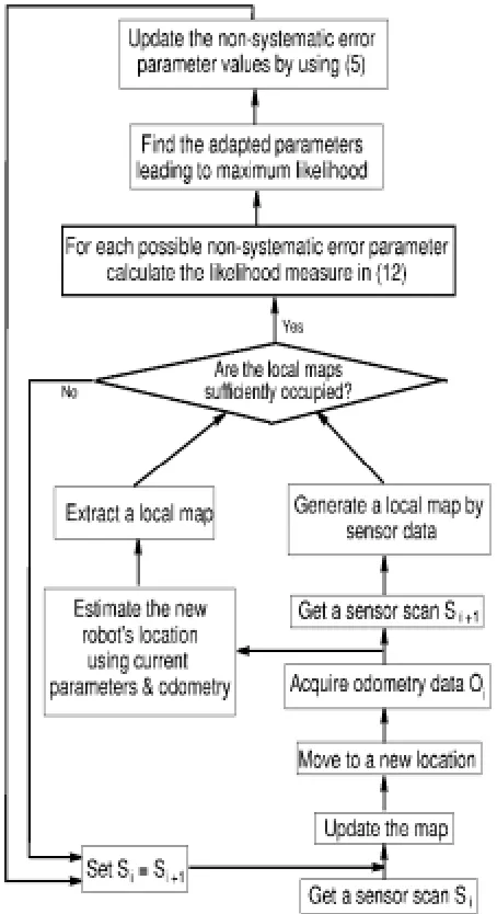
in (12) and be compared to the local map, generated from the recent sensor scan.7. STEP-BY-STEP ALGORITHM
Figure 4 demonstrates a step-by-step algorithm of our calibrated pose estimation method while the robot is exploring and mapping the environment around itself. It acquires a sensor scan
S
i at thei
thiteration. By using the recently obtained sensory data it updates a global occupancy grids map, that has been gradually created by employing a map building method e.g. Bayesian method [15,16], Dempster-Shafer reasoning [19] method or pseudo information method [17,18]. The robot moves to a new location in the next step (i+1thiteration). It acquires the odometry data
O
i and gets a new sensor scanS
i+1. The robot is able to create a local map, merely by the new sensory data (without requiring any positional information). On the other hand, it estimates its new location, by making use Figure 2. A local map extracted from a global occupancyof the odometry data and calibrating its estimate by the current dead reckoning parameters
α
trans androt
α
. It uses Equation 1 without the non-systematic error terms and Equation 2 in this step. Now a local map can be extracted from the occupancy grids that are centered at the estimated position of the robot. This map is calculated in the same size of the local map that is generated from sensory data. In the next step, the two maps are checked if they satisfy the sufficient occupancy criterion. If they do not, algorithm skips to the next iteration by settingS
i=
S
i+1 and updating the map etc. Otherwise, for each possible(
α
*trans(i),
α
rot*(i))
T value, the new robot's pose is re-estimated and the corresponding local map is re-extracted and the fitness measuref
( )
Γ
,
Γ
'
is calculated by (12). The parameter values, which lead to maximum fitness and hence to maximum likelihood, are chosen as) i *( rot ) i *( trans
,
α
α
and applied to Equation 5 to adapt αtrans andα
rot values in the next step. Finally, the next iteration is started by replacingS
i withS
i+1 and updating the map etc.8. EXPERIMENTS
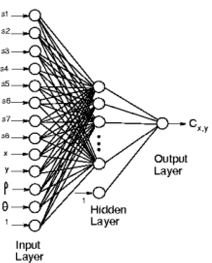
Khepera miniature mobile robot has been applied to exploration, localization and map building experiments. In these experiments, the data provided by 8 infrared sensors around Khepera, were the only sources of information (See [14] or [20] for more details on Khepera sensors and structure). There is no accurate inverse model for the infrared proximity detectors, like the model for ultrasonic range finders [21]. We trained a feed-forward multi-layered perceptron to implement an inverse model for the sensors. The inputs of the network are the eight proximity values, and the local coordinates of a cell in the occupancy grids map around the robot. The output of the network is the occupancy probability value of the cell.
The architecture of the neural network is shown in Figure 5. This output value is fused with the associated occupancy probability value of the same cell in a global map of the environment. This global map has been calculated based upon
Figure 4. Our proposed step-by-step algorithm of calibrated pose estimation for a mobile robot, while it is exploring and mapping the environment around itself.
resulting probability is applied to improve the global map. In other words, during exploration of the environment by the reactive obstacle avoidance method of Braitenberg [22], Khepera creates a local occupancy grids map in every sensing iteration. These local maps are integrated with an initially blank global map and it improves gradually. Another more intelligent alternative for obstacle avoidance is our newly introduced method of fuzzy rule-based command fusion [23].
Figure 5. The feed-forward perceptron that was trained for local map building, by using proximity data, provided by Khepera's infrared sensors.
Figure 6. A photo of khepera and the environment, in our experiments.
our experiments have been done. The well-known UMBmark (University of Michigan Benchmark) was tried in the first experiment. The robot travels a square path with a perimeter of 200cm length, 16
times in clockwise and 16 times in counterclockwise direction.
Figure 7 shows the occupancy grids map, created by pseudo information fusion, and the square path inside it. Practically, the robot does not travel the exact square path in each round, because the motion control commands are created based on the robot's pose information, acquired from the erroneous odometry data. It causes the robot not to return to its initial starting point in each round. This deviation of the location of the robot with respect to the original point of motion starting was manually measured. In the first trial of 32 rounds, their mean values were
∆
x
=
35
.
5
mm and3 . 26
=
∆y mm, equivalent to a relative error of 2.21%. This relative error is computed by
(
x y)
( )
4L %100 × ∆ 2 +∆ 2 where L=50mm is the side length of the square path. The UMBmark calibration parameters were calculated to be
9991
.
0
E
d=
andE
b=
0
.
9953
. They are some correction factors for wheel diameter and wheelbase, respectively. They were computed, based on the results that were obtained in the first trial, in order to decrease the systematic odometry error (Refer to [3] for more details on UMBmark basics and formulation). In the second trial, the calibrated values of the wheel diameter and base were applied to odometry and motion command generation process. This calibration caused a lower average deviation of∆
x
=
15
.
3
mm and ∆y=12.8mm, or in other words a relative error of 0.99%. In the third trial, we applied our proposed calibration method to the pose estimation and motion commands generation. It was observed that the robot traverses the square path more accurately and the average position deviation was measured as∆
x
=
3
.
2
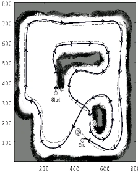
mm and ∆y=1.6mm. This is equivalent to a relative error of 0.178%. It is seen that relative estimation error has decreased by 82%.Figure 7. The square path, traveled by the robot in our UMBmark experiment.
point that was actually reached by the robot is located in a far distance from the estimated end point and following errors were measured:
mm
168
|
y
y
|
|
y
|
mm
269
|
x
x
|
|
x
|
Path Estimated End
Path Estimated End
=
−
=
∆
=
−
=
∆
At the same experiment, the same odometry data were applied to our proposed calibrated version of dead reckoning method and another estimation for the path was obtained. Both the actual and the new estimated paths are depicted in Figure 9. In contrast with the previous case, it is observed that the estimated path is much closer to the real one. That is because of the efficient calibration of systematic error of odometry data by using the adapting parameters
α
*trans andα
*rot. Indeed, end position estimation errors were measured as below:mm
38
|
y
y
|
|
'
y
|
mm
25
|
x
x
|
|
'
x
|
Path Estimated End
Path Estimated End
=
−
=
∆
=
−
=
∆
Thus, estimation error has been reduced by:
Figure 8. Solid and dash lines show the real and the estimated paths, traversed by the robot respectively.
% 66 . 85 % 100 |
| | |
| ' | | ' | 1
2 2
2 2
= ×
∆ + ∆
∆ + ∆ −
y x
y x
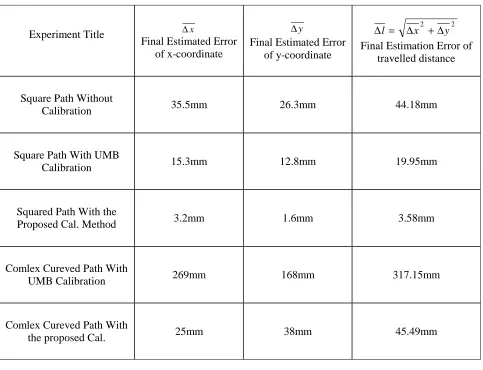
Table 1 shows the summary of the experimental results.
9. CONCLUSIONS
A new approach for calibration of dead reckoning process in pose estimation of mobile robots was proposed in this paper. We attempted to model the systematic part of the error, existing in odometry data, by introducing two calibration
parameters and estimating them adaptively. It was suggested to fuse the current sensory and odometry information with the information that had been obtained previously. The local map, generated by current sensory data, is integrated with a local map that is extracted from a global occupancy grids map of environment. Actually, the most desired parameters are those, which lead to a mostly fitted version of an extracted local map. It was shown that the proposed approach gives a maximum likelihood estimation of the parameters. The most important advantages of the method are its simplicity and its applicability to the cases where the robot is equipped with short-range distance sensors TABLE 1. Summary of the Experimental Results.
Experiment Title ∆x
Final Estimated Error of x-coordinate
y
∆
Final Estimated Error of y-coordinate
2 2
y x
l = ∆ +∆
∆
Final Estimation Error of travelled distance
Square Path Without
Calibration 35.5mm 26.3mm 44.18mm
Square Path With UMB
Calibration 15.3mm 12.8mm 19.95mm
Squared Path With the
Proposed Cal. Method 3.2mm 1.6mm 3.58mm
Comlex Cureved Path With
UMB Calibration 269mm 168mm 317.15mm
Comlex Cureved Path With
(proximity detectors). In our experiments, Khepera robot was utilized to examine the performance of the method for reduction of pose estimation error. The proximity data, provided by the infrared sensors of the robot and the odometry data, provided by wheel encoders, were the only sources of information in these experiments. Results show that our approach causes a reduction of more than 80% in pose estimation error. Besides, the proposed approach is applicable in an online case. It means that the robot may calibrate its position by this method, while it is exploring the environment around itself and mapping it. In this case, the important difference is the fact that there is no previously created global map for extraction of local maps. But it seems very probable that a partially generated map can be useful to be applied in our method.
10. ACKNOWLEDGEMENT
This research work was supported through mutual research program between University of Tehran, Faculty of Engineering (IRAN) and University of the Ryukyus, Faculty of Engi neering, Department of Information Engineering (JAPAN) by Monbusho scholarship scheme.
11. REFERENCES
1. An, C. H. and Atkeson, C. G. and Hollerbach, J. M., “Model Based Control of a Robot Manipulator”, The MIT Press, Cambridge, MA, (1988).
2. Cox, I. J. and Wilfong, G. T., “Autonomous Robot Vehicles”, Springer Verlag, (1990).
3. Borenstein, J. and Everett, H. R. and Feng, L., “Where Am I? Sensors and Methods for Mobile Robot Positioning”, Technical Report, University of Michigan, ftp://ftp.eecs.umich.edu/ people / johannb / pos96rep.pdf, (1996).
4. C r o wl ey, J . L. , “M at h emat i cal F o u n d at i o n s o f Navigation and Perception for an Autonomous Mobile Robot”, In Reasoning with Uncertainty in Robotics Edited by L. Dorst, M. Van Lambalgen and F. Voordraak, Volume 1093 of Lecture Notes in Ar t i fi ci al I n t el l i gen ce, 9 - 5 1 , S p r i n ger V er l ag, (1995).
5. Thrun, S., Burgard, W. and Fox, D., “A Probabilistic
Approach to Concurrent Mapping and Localization for Mobile Robots”, Machine Learning, 31, 29-53, (1998)
6. Abidi, A. and Gonzalez, R. C., “Data Fusion in Robotic and Machine Intelligence”, Academic Press, (1992).
7. Dasarathy, B., “Decision Fusion”, IEEE Press, (1994).
8 . R i c h r d s o n , J . M . a n d M a r s h , K . M . , “ F u s i o n o f M u l t i s e n s o r D a t a ” , I n t e r n a t i o n a l J o u r n a l o f R o b o t i c s, V o l u me 7 , N u mb e r 6 , ( 1 9 8 8 ) , 7 8 -9 6 .
9. Van Dam, J. W. M., “Environment Modeling for Mobile Robot: Neural Learning for Sensor Fusion”, University of Amsterdam, P h.D. Thesis, (1998).
10 . M a c K e n z i e , P . a n d D u d e k , G . , “ P r e c i s e P o s i t i o n i n g U s i n g M o d e l - B a s e d M a p s ” , P r o c e e d i n g s I E E E I n t e r n a t i o n a l C o n f e r e n c e o n R o b o t i cs a n d A u t o m a t i o n, S an D i ego , C A, ( 1 9 9 4 ) .
1 1 . T h r u n , S . , “ L e a r n i n g M a p s f o r I n d o o r M o b i l e R o b o t N a v i g a t i o n ” , A r t i f i c i a l I n t e l l i g e n c e, ( 1 9 9 8 ) .
1 2 . T h r u n , S . , “ A n A p p r o a c h t o L e a r n i n g M o b i l e R o b o t N a v i g a t i o n ” , R o b o t i c s a n d A u t o m a t i o n S y s t e m s, 1 5 , 3 0 1 - 3 1 9 , ( 1 9 9 5 ) .
13 . F o l ey, J . an d V an D am, A. an d F ei n er , S . an d H u g h e s , J . , “ I n t e r a c t i ve C o mp u t e r Gr a p h i c s : P r i n c i p l e s a n d P r a c t i c e ” , A d d i s o n - W e s l e y , ( 1 9 9 0 ) .
14. K-Team, S. A., “Khepera User Manual (Fifth Edition)”, Lausanne, Switzerland, (1998).
15. Elfes, A., “Using Occupancy Grids for Mobile Robot Perception and Navigation”, Computer, 22(6), 249-265, (1989).
16. Elfes, A., “Sonar-Based Real-World Mapping and Navigation”, IEEE Journal of Robotics and Autom ation, 249-265, (1987).
17 . As h ar i f, M . R . an d M o s h i r i , B . an d H o s ei n N e z h a d , R . , “ P s e u d o I n f o r m a t i o n M e a s u r e : A N ew C o n cep t fo r S en s o r D at a F u s i o n , Ap p l i ed in Map Building for Mobile Robots”, Proceedings of International Conference on Signal Processing Applications and Technology (ICSPAT 2 0 0 0 ), D a l l a s , T e x a s , U S A , 1 6 - 1 9 O c t o b e r ( 2 0 0 0 ) .
18. Asharif, M. R. and Moshiri, B. and Hosein Nezhad, R., “Environment Mapping for Khepera Robot: A New Method by Fusion of Pseudo Information Measures”, Proceeings of International Symposium on Artificial Life and Robotics (AROB), Tokyo, Japan, January (2001).
19. Murphy, R., “Dempster-Shafer Theory for Sensor Fusion in Autonomous Mobile Robots”, IEEE Transactions on Robottics and Automation, Vol. 14, No. 2, (1998).
Japan, (October 1993), 501-513.
21. Oriolo, G. and Ulivi, G. and Vendittelli, M., “Fuzzy Maps: A New Tool for Mobile Robot Perception and Planning”, Journal of Robotic Systems, Volume 14, Number 3, (1997), 179-197.
2 2 . B r a i t e n b e r g , V . , “ V e h i c l e s ” , K l u w e r A c a d e mi c
Publishers, (1984).