A SUB
-LOADING SURFACE MULTILAMINATE MODEL
FOR ELASTIC-PLASTIC POROUS MEDIA
S. A. Sadrnejad
Department of Civil Engineering, K.N.Toosi University of Technology Teheran, Iran, sadrnejad@hotmail.com
(Received: May 26, 2002 – Accepted in Revised Form: October 3, 2002)
Abstract A framework for development of constitutive models based on semi-micromechanical aspects of plasticity is proposed. The resulting of this model for material employed friction type failure criterion, sub-loading surface, and associated flow rule. This model is capable of predicting effects of the rotation of principal stress/strain axes and consequent plastic flow, induced anisotropy of strength, particularly, in cyclic loading. Also, this model has the potential of predicting the behavior of fully inherent anisotropic material, and strain history distributions at a point up to failure. The predicted model results and their conformity with experimental results of cyclic loading including the pre-failure specifications show the capability of the mode.
Key Words Multi-Laminate Framework, Sub-Loading Surface Model, Elastic-Plastic, Cyclic Loading
ﻩﺪﻴﻜﭼ
ﻩﺪﻴﻜﭼ
ﻩﺪﻴﻜﭼ
ﻩﺪﻴﻜﭼ
ﺑﺏﻮﭼﺭﺎﻬﭼﻚﻳ ﺮ
ﺎﺳﺍﻂﺑﺍﻭﺭﻪﻌﺳﻮﺗﻱﺍ
ﺮﺑﺎﻬﻟﺪﻣﻲﺳ ﺍﻩﺪﺷﻪﺋﺍﺭﺍﻲﻨﻴﺑﻩﺭﺫﻪﻤﻴﻧﻱﺮﻴﻤﺧﻱﺭﻮﺌﺗﻪﻳﺎﭘ
ﺖﺳ . . . .
ﺭﺎﺘﻓﺭﻱﺍﺮﺑ ﺩﺍﻮﻣ
ﺎﺗﻙﺎﻜﻄﺻﺍﺎﺑ
ﻪﻧﺎﻴﺷﺁﻝﺪﻣﺖﺴﻜﺷ ﻪﻠﺣﺮﻣ ﺎﺑﻱﺍ
ﺮﻳﺯﺢﻄﺳ
ﺖﺳﺍﻩﺪﺷﻪﺋﺍﺭﺍﻱﺭﺍﺬﮔﺭﺎﺑ .
ﻝﺪﻣﻦﻳﺍ
ﺶﻴﭘ ﺖﻴﻠﺑﺎﻗ ﺭﺎﺛﺁﻲﻨﻴﺑ
ﻭﺶﻨﺗﻲﻠﺻﺍ ﻱﺎﻫﺭﻮﺤﻣﺶﺧﺮﭼ ﻭﺶﻧﺮﻛ
ﺎﻧ
ﺭﺩﺹﻮﺼﺨﺑ ﺖﻣﻭﺎﻘﻣﻲﻠﻴﻤﺤﺗﻲﻧﺎﺴﻤﻫ ﺮﺛﺍ
ﺩﺭﺍﺩﺍﺭﺏﻭﺎﻨﺘﻣﻱﺭﺍﺬﮔﺭﺎﺑ .
ﺭﻲﻨﻴﺑﺶﻴﭘﻞﻴﺴﻧﺎﺘﭘﻝﺪﻣﻦﻳﺍﻦﻴﻨﭽﻤﻫ ﻓ
ﺭﺎﺘ ﺍﻮﻣ ﺎﺑﺩ ﺎﻧ
ﻪﭽﺨﻳﺭﺎﺗﻊﻳﺯﻮﺗﻭﻲﺗﺍﺫﻲﻧﺎﺴﻤﻫ
ﺮﻫﺭﺩﺶﻧﺮﻛﻲﻧﺎﻣﺯﻱﺎﻫ ﺎﺗﻪﻄﻘﻧ
ﺍﺭﺖﺴﻜﺷﻪﻠﺣﺮﻣ ﺩﺭﺍﺩ
.
ﻭﻝﺪﻣﻩﺪﺷﻲﻨﻴﺑﺶﻴﭘﺞﻳﺎﺘﻧ ﻱﺭﺍﺬﮔﺭﺎﺑﻱﺍﺮﺑﻥﺁﻖﻴﺒﻄﺗ
ﺎﺑﻩﺍﺮﻤﻫﺏﻭﺎﻨﺘﻣ ﻩﮋﻳﻭ
ﺖﺳﺍﻝﺪﻣﺖﻴﻠﺑﺎﻗﺪﻳﻮﻣﺖﺴﻜﺷﺯﺍﻞﺒﻗﻱﺭﺎﺘﻓﺭﻱﺎﻬﻴﮔ .
1. INTRODUCTION
Constitutive modeling of material plasticity including different features has been the subject of numerous investigations during the recent years, primarily because of the increasing awareness of complexity of the loading conditions to which soil structures are subjected and the corresponding need for more accurate analysis for prediction of safety of such structures. The parallel development of more powerful and efficient numerical methods of analysis has motivated and allowed the use of sophisticated constitutive models beyond the linear or simple nonlinear elastic-plastic constitutive laws which were utilized in the early stages.
Most models proposed are based on the theory of elastic-plasticity, incorporating different yield criteria, flow and hardening rules. Strain hardening models according to various isotropic, kinematics or mixed hardening rules have been proposed.
These models usually deal with a single or a combination of stress invariant. Rotation of the direction of principal axes of either stress/strain or both has been observed in many tests. A model based on invariant of stress/strain tensors, therefore cannot cope with the real behavior of soil under a complex loading program while either the values of stress or strain invariant are kept constant. The task of representing the overall stress tensor in terms of micro level stresses and the condition, number and magnitude of contact forces has long been the aim of numerous researchers [1-3]. Sadrnejad developed a multi-laminate model for granular materials [4,5].
stress, characterization of cohesion and fabric, representation of kinematics, development of local rate constitutive relations and evaluation of the overall differential constitutive relations in terms of the local quantities.
Properly prediction of soil behavior under cyclic loading is a major practical problem in geo-mechanics. In reality, stress/strain relation for soil under cyclic loading depends on many objects. Therefore, without using this task mathematical models will be impossible. Prof. K. Hashigushi proposed the first sub-loading model in 1989 [6]. Many progress and development implemented on this model later [7-9]. Capability of this model encouraged the author to build up a new model based on multi-laminate framework adding all advantages of both.
In this paper, a multi-laminate based model capable of predicting the behavior of soils on the basis of sliding mechanisms and elastic behavior of particles has been presented. The capability of the model is to predict the behavior of soil under arbitrary stress paths. The influences of rotation of the direction of principal stress axes and induced anisotropy are included in a rational way without any additional hypotheses.
2. BASIC ASSUMPTIONS AND DISCUSSIONS
Multi-laminate framework defined by small continuum structural units formed as an assemblage of particles and voids filling infinite spaces between the sampling planes, has appropriately justified the contribution of interconnection forces in overall macro-mechanics. Plastic deformations are assumed to occur due to sliding as shearing, separation/closing of the boundaries as volume change. Elastic deformations are the overall responses of structural unit bodies. Therefore, the overall deformation of any small part of the medium is composed of total elastic response and an appropriate summation of sliding, separation/closing phenomenon under the current effective normal and shear stresses on sampling planes.
3. THE CONSTITUTIVE EQUATIONS
The classical decomposition of strain increments
under the concept of elastic-plasticity in elastic and plastic parts are schematically written as follows:
p e d d
dε= ε + ε (1)
The increment of elastic strain (dεe) is related to the increments of effective stress (dσ′) by:
' 1 e e [D ] .d
dε = − σ (2)
Where, [De ]-1 is elastic compliance matrix, usually assumed as linear and is obtained as follows:
) (
G )
G 3 2 K ( ijkl
De = − δijδkl+ δikδjl+δilδjk (3)
Where, K and G are bulk modulus and the shear modulus, respectively.
To obtain plastic strain increments (dεp), for the soil mass, the stress-strain increments relation, is expressed as:
' p p C .d
dε = σ (4)
Where, Cp is plastic compliance matrix.
Clearly, it is expected that all the effects of plastic behavior be included in Cp. To find out Cp, the constitutive equations for a typical slip plane must be considered in calculations. Consequently, the appropriate summation of all provided compliance matrices corresponding to considered slip planes yields overall Cp, therefore, strain increment at each stress increment is calculated as follows:
' n
1 i
p i T i
p { W[L ] .C .[L ]}.d n
1
dε =
∑
ε σ σ=
(5)
Where, Lε and Lσ are transformation matrices for strain and stresses, respectively and n is number of planes.
To satisfy conditions of applicability of the theory from the engineering viewpoint and also to reduce the extremely high computational costs, a limited number of necessary and sufficient sampling planes are considered.
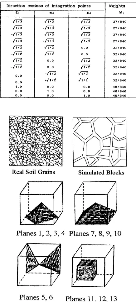
through the media and avoiding huge computing time is a fair number. The orientation of the sampling planes as given by their direction cosines and the weight coefficients for numerical integration rule are given in first three and the last columns of Table 1.
The coefficients Wi are simply calculated based on Gauss Quadrature numerical integration rule. A coordinate system has been employed for each plane in such manner that one axis is perpendicular to the plane and the other two are on the plane. Plastic shear strain increments on each plane is considered as two component vectors on defined coordinate axes of plane. Thirteen sets of direction cosines of coordinate axes are presented in Table 1.
One of the important features of multi-laminate framework is that it enables identification of the active planes as a matter of routine. The application of any stress path is accompanied by the activities of some of the 13 defined planes in three-dimensional media. The values of plastic strain on all the active planes are not necessarily the same. Some of these planes initiate plastic deformations earlier than the others. These priorities and certain active planes can change due to any change of direction of stress path, a number of active planes may stop activity and some inactive ones become active and some planes may take over others with respect to the value of plastic shear strain. The first set of planes, indicating %10 shear strain can be identified together as the first mode of failure. Thus, the framework is able to predict the mechanism of failure. Figure 2 shows the orientation of all 13 planes in similar cubes. In order to clarify their positions, they have been presented in four cubes.
TABLE 1. Direction Cosines and Weight Coefficients of Integration Points.
Figure 1. The orientation of 13 planes, real grains and assumed blocks
4. CONSTITUTIVE EQUATIONS FOR A SAMPLING PLANE
A sampling plane is defined as a boundary surface, which is a contacting surface between two structural units of polyhedral blocks. These structural units are parts of an inheterogeneous continuum and for simplicity they are defined as a full homogeneous and isotropic material. Therefore, all inheterogeneities behavior is supposed to appear in inelastic behavior of corresponding slip planes. Figure 1 shows these defined planes (say 13). The number of planes may be chosen as any number, however, based of some numerical experiences, 13 is found to fit a rationally justified and got enough power to show any distribution through the material.
5. SUBLOADING AND NORMAL YIELD SURFACES
The normal yield surface is defined here as a limiting boundary surface which separate possible and impossible cases in stress domains. This boundary is also a function of hardening parameters.
The sub-loading surface is a similar boundary except that, it is smaller and positioned any where inside normal yield surface. This boundary always passes through stress position and its size may change. The mobility of this surface is controlled by a center of similarity. The center of similarity moves when plastic strains take place. For an isotropic and homogeneous material sub-loading surfaces for all planes are the same. However, different plastic strains of planes, induced anisotropy provided in material and also different shape and position of sub-loading surfaces is obtained. Every plane has its normal yield surface, which is usually defined as effective stress
σ
, ,
xiσ
σ
'yi '
zi '
space, which are effective stress components on ith plane. Figure 2 shows sub-loading and normal yield surfaces of one plane. Normal yield surface for ith plane is defined as follows:
0
)
(
)
ˆ
(
′
−
F
H
i=
f
σ
(6)i i
i
σ
α
σ
ˆ
′
=
′
−
ˆ
(7)where
)
/
ˆ
(
ˆ
)
ˆ
(
2 *m
2f
σ
i′
=
σ
ni′
+
σ
i (8)2 2
2 *
) ˆ ˆ ( ) ˆ ˆ ( ) ˆ ˆ (
ˆi σ xi σni σ yi σni σ zi σ ni
σ = ′ − ′ + ′ − ′ + ′ − ′
(9)
zi yi i
mi
σ
σ
σ
σ
ˆ
′
=
ˆ
′
+
ˆ
′
+
ˆ
′
(10)Where,
f
(
σ ′
ˆ
i)
is normal yield function,σ ′
ˆ
istress vector comprisingσ
ˆ
′
xi,
σ
ˆ
′
yiand
σ
ˆ
zi′
for ith plane, also scalar Hi andα
ˆ
istand for isotropic hardening parameter and kinematics hardening vector respectably.σ
ˆ
ni′
and
σ
ˆ
i′
* are the effective normal and shear stresses on ith plane respectably.m is defined as a constant material property.
f
(
σ ′
ˆ
i)
is a homogeneous elliptical function in*
ˆ
~
ˆ
niσ
iσ
′
′
plane, and the ratio of two diameters of the ellipse remains constant while plasticity is in progress.6. HARDENING RULE
An isotropic shear-hardening rule is employed to carry any change of normal yield surface size during plasticity on ith plane. F(Hi) introduced as hardening function for ith plane, is defined as follows:
F Hi
(
)
=
F [1 + b
oi i(
1
−
e
−di Hi.)]
(11) where,2 2
2
) 3 (
) 3 (
) 3 (
i v d i z d i v d i y d i v d i x d H
p
p p
p p
p
i
ε ε ε
ε ε
ε − + − + −
=
(12)
d
ε
vip is plastic volumetric strain, Foi is initial value of F, and both di and bi are two isotropic hardening parameters, all corresponding to ith
A kinematics hardening is also employed to obtain only the changes of position of normal yield surface center. The following functions represent this rule:
i i i i
I
B
A
σ
σ
α
ˆ
′
=
+
ˆ
(13)Where, I is unity matrix, A, and B are parameters of plastic deformations which in this model are as follows:
A = 0 (14)
B
=
K
iH
iMi. H
i (15)Ki and Mi are constant parameters of hardening for
ith plane.
It can be concluded that
α
ˆ
i and Hi are two first order homogeneous functions of plastic strain increment. However, they can be formed as follows:i i
λ
a
α =
ˆ
′
(16)H
i= h
λ
i (17)Where, vector ai and scalar hi are related to stress and plastic strain variations. ai is calculated as follows: i i i M i i
i
K
H
h
a
iσ
σ ′
=
.
.
ˆ
(18)7. FLOW RULE AND CONSISTENCY CONDITION
Flow rule is expressed as follows:
d
ε
ip=
λ
i.
n
i (19)Where ni is the vector for orientation of plastic strain increment. The equation of loading surface for ith plane is written as follows:
)
ˆ
,
H
,
(
σ
iσ
i′
=
ii
Q
Q
(20)However, the consistency condition is obtained as:
0
=
ˆ
+
H
+
)
(
i iα
i∂α
∂
∂
∂
σ
∂σ
∂
i i i i i iQ
H
Q
Q
tr
(21)λ
∂
∂σ
σ
∂
∂
∂
∂α
i i i i i i i itr
Q
Q
H
Q
a
=
−
(
)
(
h +
)
i
i
(22)
Therefore, parameter Di is defined as follows:
D
Q
H
Q
a
Q
i i i i i i i i=
−
(
∂
)
∂
∂
∂α
∂
∂σ
h +
i(23)
The plastic strain increment is obtained by the following equation:
λ
ii i
i
tr n T
D
=
(
.
)
(24)where
n
Q
Q
i i i i i=
∂
∂ σ
∂
∂ σ
(25)From Equations 25, 20, and 19 the characteristic equation is obtained.
d Q Q D Q i p i i i i T i i i ε ∂ ∂ σ ∂ ∂ σ ∂ ∂ σ σ = [ ( ) ) ] ( d i 2 (26)
Generalizing the rule for normal yield surface and loading surface, it is adopted that:
i 2
]
d
)
(
)
(
[
σ
∂σ
∂
∂σ
∂
∂σ
∂
ε
i i i T i i i i p if
D
f
f
which is based on:
)
F(H
-)
ˆ
f(
=
)
ˆ
,
H
,
(
σ
i iα
iσ
i′
iQ
(28)then,
C
Q
Q
D
Q
i p i i i i T i i i=
[
(
)
)
]
∂
∂ σ
∂
∂ σ
∂
∂ σ
(
2 (29)
C
ip as a whole, represent the plastic resistance corresponding to the ith plane and must be summed up as the contribution of this plane with the others. The scalar value of Di for the ith plane is calculated as follows:}] ˆ R U ) x Sˆ -R ˆ )( R 1 ( c a ˆ . h ) H ( nF ) H ( F { n [ tr D i i i i i i i i i i i i i i i σ + σ − + + σ ′ = (30) where
F H
' (
i)
=
F b d e
oi. .
i i.
−d Hi. i (31)hi in general, hi is a function of plastic deformation. For simplicity, it is taken constant for all planes and equal to
( / )
2 3
0 5. . As already stated, the normal yield surface is a homogeneous function. Therefore, n is equal to one. ni is a 3x1 vector as follows:T zi i yi i xi i 5 . 0 zi i yi i xi i T zi yi xi i ] f f f [ ] f f f [ } n , n , n { n ∂σ ∂ + ∂σ ∂ + ∂σ ∂ ∂σ ∂ + ∂σ ∂ + ∂σ ∂ = = − (32)
{
xi yi zi}
I
σ
σ
σ
σ
ˆ
=
ˆ
,
ˆ
,
ˆ
(33)S
i=
{
S
xi, S , S
yi zi}
(34)where, Sxi, Syi, and Szi are components of center of similarity vector for the ith plane.
i
ˆ
-
α
ii
S
S
)
=
(35)i i
i
σ
α
σ
ˆ
=
−
ˆ
(36){
}
T zi yi xii
α
α
α
α
ˆ
=
ˆ
,
ˆ
′
ˆ
(37)Where,
α
ˆ
xi,
α
ˆ
yiandα
ˆ
zi are components of the center of normal yield surface vector for the ith plane.Ri is calculated for when n=1 as follows:
R
B
B
AD
A
i
=
+
+
[
(
2)
0 5.]
(38)
where
A
=
m F
2[
2(
H
i)
- f
2(
S
)
i)]
(39)) Sˆ Sˆ )( ˆ ˆ ( ) Sˆ Sˆ ( ) ˆ ˆ ( ) Sˆ Sˆ ( ) ˆ ˆ ( Sˆ . ˆ m B mi zi mi zi mi yi mi yi mi xi mi xi mi mi 2 − σ − σ + − σ − σ + − σ − σ + σ =
and D=[m.f(σ)i)]2 (40)
The value of Ui is calculated as follows:
i i S i i i
R
R
R
u
U
iˆ
.
)
1
(
1 −=
(41)where Si and ui are two constant parameters which must be known by calibrating the model. Also, Ri is found as follows:
)
(
)
ˆ
(
ˆ
i i iH
F
f
R
=
σ
(42)8. IDENTIFICATION OF PARAMETERS
In a general case, for the most anisotropic, non-homogeneous material, 13 sets of material parameters corresponding to plastic sliding of each sampling planes are required. However, any knowledge about the similarity of the sliding behavior of different sampling planes reduces the number of required parameters.
(i.e. E and ν) correspond to elastic behavior of soil skeleton. The value of m is obtained through calibration of drained test corresponding to εv(volumetric strain) versus ε1(major axial strain). The values of b, d, k, and M are obtained through the variation of deviatoric stress versus axial strain. The parameters u and s are obtained through calibration of additive deformations in cyclic response of material. The dimension of hysteresis loop depends on parameters c and x.
The initial conditions which are to be define for the model are:
σo (initial stresses), εo (initial strains) Fo, (initial value of normal yield surface),
α
ˆ
0(initial position of normal yield surface center), so (initial position of the center of similarity). σo and εo are normally defined through initial and boundary conditions. The initial value of Fo depends on σno (initial normal stress on plane) and loading type. The values ofα
ˆ
0 depend on inherent anisotropy condition of each plane. This parameter can define the orientation of normal to plane regarding the fabric orientation of material at corresponding point. However, for the isotropic material it is as follows:φ
α
α
α
ˆ
0x=
ˆ
0y=
ˆ
0z=
(43)The parameter Co depends on the degree of
pre-consolidation in material. It increases with the higher degree of pre-consolidation.
9. RESULTS
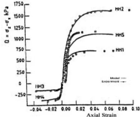
To present the capabilities of the proposed model the experimental results [10], which were obtained from, hollow cylindrical and true triaxial cube tests on Hostun sand are considered with the model results. The eleven model parameters for this comparison were obtained through calibration and are show in Table 2.
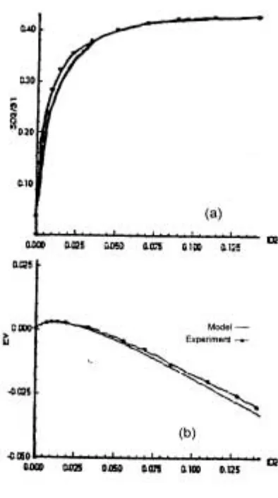
Figures 3 and 4 are the results of calibrating the model with experiments. Figure 3 is the variation of Q (Q = σz - σx) versus εz for extension, compression and cyclic loading. Figure 4 is the variation of εv (εv= ε1+ε2+ε3) versus ε1, which corresponds to the previously mentioned tests. Three invariant SD2, S1, and ID2 are defined as follows:
SD2
3 1 2
2
2 3 2
3 1 2
= 1[(σ −σ ) +(σ −σ ) +(σ −σ ) ] (44)
3 2 1
1
=
σ
+
σ
+
σ
S
(45)] ) ( ) ( ) [( 3 1
2 2
1 3 2 3 2 2 2
1 ε ε ε ε ε
ε − + − + −
=
ID (46)
TABLE 2. Parameter Values.
Figures 5 to 9 show comparison of model results with tests CH1.TST, CH2.TST, CH3.TST, CH4.TST, and CH5.TST respectively. Figures 10
and 11 are results corresponding to PHH3B.TST and PHH3C.TST, which were required to be predicted and presented at the conference in Cleveland [11]. The variations of τ versus γ and εv versus γ are presented and compared with experimental results. The foregoing prediction of test results is encouraging and shows the validity of the model.
10. CONCLUSIONS
From this study a model capable of predicting the behavior of granular material on the basis of sliding mechanisms and elastic behavior of particles has been presented. The concept of multi-laminate framework has been applied successfully on a high Figure 4. Calibration results.
Figure 5. test CH1.
level sub-loading surface model for granular materials. The predicted numerical results show good agreement
with the observed behavior of sand specimens tested in hollow cylindrical, true tri-axial test, and Figure 9. Test CH5.
Figure 10. Test PHH3. Figure 7. Test CH3.
also complex stress path cyclic loading conditions. The influence of rotation of the directions of principal stress axes is included in a rational way without any additional hypotheses. The behavior of sand has been modeled based on a semi-microscopic concept, which is very close to the reality of particle movement in soils. Accordingly, the sampling plane constitutive formulations provide convenient means to classify loading event, generate history rules and formulate independent evolution rules for local variables. This is an advantage of the model including induced anisotropy in plastic behavior of materials.
11. ACKNOWLEDGMENT
The author would like to express his gratitude to Prof. K. Hashigushi for his helpful guidance and providing many valuable suggestions.
12. REFERENCES
1. Christofferson, C., Mehrabadi, M. M. and Nemat Nasser, S., “A Micro Mechanical Description of Granular Behavior”, J. Appl. Mech., 48, (1981), 339-344.
2. Konishi, J., “Microscopic Model Studies on the Mechanical
Behavior of Granular Materials”, Proc. U.S. Japan Seminar on Continuum Mechanical and Statistical
Approaches in the Mechanics of Granular Materials,
(Eds. S. C. Cowin and M. Satake), Gakujutsu Bunken Fukyukai, Tokyo, (1978), 27-45.
3. Nemat Nasser, S. and Mehrabadi, M. M., “Stress and Fabric in Granular Masses”, Mechanics of Granular Materials: New Models and Constitutive Relations, (Eds. J.T. Jenkins and M. Satake), Elsevier Sci. Pub., (1983), 18.
4. Sadrnejad, S. A., “Multilaminate Elastoplastic Model for Granular Media”, Journal of Engineering, Tehran, Iran, No. 182, (1992), 11-24.
5. Sadrnejad, S. A. and Pande, G. N., “A Multilaminate Model For Sand”, Proceeding of 3rd International
Symposium on Numerical Models in Geomechanics,
NUMOGIII, 811 May, Niagara Falls, Canada, (1989). 6. Hashiguchi, K., “Subloading Surface Model in
Unconventional Plasticity", Solids Structure, Vol. 25, No. 8, (1989), 917-945.
7. Hashiguchi, K., “Fundamental Requirements and Formulation of Elastoplastic Constitutive Equation with Tangential Plasticity", Kyushu Univ., (1993).
8. Hashiguchi, K., “Constitutive Equation of Soils Based on the Subloading Surface Concept", J. Fac. Agr., Kyushu Univ., 39(1.2), (1994), 91-103.
9. Hashiguchi, K., “Mechanical6 Requirement and Structures of Cyclic Plasticity Models", Int. J. of Plasticity, Vol. 9, (1993), 721-728.
10. International Workshop on Constitutive Equations for Granular Non-Cohesive Soils, Information Package, Case Western Univ. Cleveland, (July 1987), 22-24.