Optimum Drill Bit Selection by Using Bit Images and Mathematical Investigation

Please cite this article as: M. Momeni, S. Ridha, S. J. Hosseini, X. Liu, A. Atashnezhad, S. Ghaheri, Optimum Drill Bit Selection by Using Bit Images and Mathematical Investigation, International Journal of Engineering (IJE), TRANSACTIONS B: Applications Vol. 30, No. 11, (November 2017) 1807-1813

International Journal of Engineering

Optimum Drill Bit Selection by Using Bit Images and Mathematical Investigation

M. Momenia_{, S. Ridha}a_{, S. J. Hosseini*}a_{, X. Liu}a_{, A. Atashnezhad}b_{, S. Ghaheri}a

a _{Department of Petroleum Engineering, Universiti Teknologi PETRONAS, Bandar Seri Iskandar, Perak Darul Ridzuan, Malaysia} b _{Department of Chemical Engineering, Oklahoma State University, Stillwater, USA}

P A P E R I N F O

Paper history:

Received 04 June 2017

Received in revised form 24 August 2017 Accepted 08 September 2017

Keywords: Bit Selection

Artificial Neural Network Image Processing Techniques Genetic Algorithm

Optimum Drilling Operation

A B S T R A C T

This study is designed to consider the two important yet often neglected factors, which are factory recommendation and bit features, in optimum bit selection. Image processing techniques have been used to consider the bit features. A mathematical equation, which is derived from a neural network model, is used for drill bit selection to obtain the bit’s maximum penetration rate that corresponds to the optimum parameters for drilling. At the end, the bit with the maximum penetration rate is chosen. The results of this study showed that bit pattern can be inserted in the calculation through a proper bit image processing technique. This is to ensure that each unique bit can be discriminated from other bits. The values of mean square error and coefficient of determination (R2_{) were respectively found as} 0.0037 and 0.9473, for the rate of penetration model. The image processing techniques were used to extract the bit features. The artificial neural network black box was converted to white box in order to extract a mathematical equation and visibility of the model.

doi: 10.5829/ije.2017.30.11b.24

1. INTRODUCTION1

A global review of wells showed that bit related cost can increase up to 40% of the well cost [1]. For a bit run, these costs include trip frequency, which is determined by the bit life or the length of the interval that the bit can keep drilling, the time-based operating cost of the drilling facility, the price of the bit and the duration of time needed to drill the interval. Consequently, this shows that drilling cost is a significant function for the life given by the bit and the rate of penetration (ROP). In turn, this means that one of the major solutions of cutting down the running cost of the bit is finding the most suitable bit design for drilling in each interval. The link between bit design and bit run performance showed that good bit selection is a crucial factor to minimize bit related cost. Accordingly, low penetration rate and short bit life will occur if the wrong bit design is chosen for the drilling condition and leads to requiring a longer time for rotating and tripping [1]. On the other hand, the bit selection program might be

*Corresponding Author’s Email: javad.hosseini@utp.edu.my (S. J. Hosseini)

impossible when the chosen well d is a wildcat well. Hence, bit selection will need to rely on seismic data which might provide the predicted thickness intervals and formation top. Trial and error methods are predominantly adopted in matching bit types to each formation. The complete list of major manufacturers’ drilling bits by Drill Bit Classifier World Oil is often used by supervisors and engineers to guide them in the field selection [2]. Furthermore, the Drill Bit Classifier also provides the most recent classification charts that

comprise of bit information along with a

performance of a bit based on the predicted drilling and geological conditions, as well as the bit design characteristics. As there are many variables that can affect ROP, including WOB, RPM, fluid viscosity and mud weight (MW), it is challenging to select a proper bit [4-6].

The artificial neural networks (ANNs) were used in some studies [7-10] to predict the IADC codes during the process of bit selection. These studies mentioned that parameters including formation properties, drilling fluid characteristics, and operational parameters are linked to the performance of the bit. Hence, they form a complicated relationship with bit performance. ANNs, with their computational intelligence, have the capacity in defining the relationship between these variables. Past studies working on neural networks have incorporated input data including rotational speed, weight on bit , drilled interval, bit size and pump rate, while bit code was considered as the output data. In their study bit code was used to consider bit features but bit codes only represent the bit name, hence, it cannot be adopted as a value for calculation.

The rock failure tests by a single row of inserts were conducted on a compound rock fracturing machine [11]. The geometrical structure of the single row of inserts is the same as one row on a roller cone bit, and its movement on the machine can reflect the true movement of inserts of a bit (Figure 1).

Different single row specimens were designed, and different types of rock samples were selected for the experiments. Figure 1 shows a rock fracturing test by a single row of the insert being conducted. Experimental results established the ability to estimate real physical distance with accuracy as high as 98.76% using image processing techniques [12]. Hence, in order to consider bit design, image processing techniques can be used as there is a strong relationship between the real size of an object and its pixels. Current bit selection methods seem problematic as they fail to consider bit features and bit pattern properly.

Figure 1. Single-row insert workpiece used to run the

indentation test [11]

Besides, the factory recommendation for safety was usually ignored during the bit selection process. In relation to this, this study applies image processing methods to properly deliberate the bit pattern. These methods were used to extract the bit features which is unique for each bit. Furthermore, during the optimization process, factory recommendations were highly considered and applied.

2. METHODOLOGY

2. 1. Image Capture Procedures To capture the bit images, this study used a 10 megapixel couple-charged device CCD camera. All of the bits were put inside a fixed box, the camera setting, and distance between the bit and the camera was kept constant. Due to the limit set for the size of images in the MATLAB® environment, the bit images were resized to 600 × 600 pixels.

A Laplacian filter with α = 1 was used to improve the edge contracts to extract the surface metrics. Structural elements were applied to clearly dilate, erode and close the boundary edges. Furthermore, a set of 1D intensity signals were generated to compute distance classifiers. These classifiers were used to characterize the most significant information from the original 2D image. The proceeding sections detail the used methods. Figure 3 illustrates an example of a bit image which the edges were enhanced by the Laplacian filter.

Figure 2. Scheme of the camera setup

2. 1. 1. First-Order Surface Metrics Ten first-order basic surface metrics, which are often used with binary images, were used to investigate the tricone rotary drill bit patterns. These metrics which were chosen as the changes in the region (ROI) generally impact the area as well as the relationship between the major and minor axes. First, using a data class converting technique, the RGB images were converted to binary class or array 0 and 1. The surface metrics obtained for each individual binary bit images were compared with a new metric as a reference image [13]. These metrics include area, which refers to the actual pixel number in the target regions, perimeter, which is the distance of the boundary surrounding each adjoining region in the image, and convex area, which refers to a number of pixels contained in the convex image (a binary image which comprises of all pixels in the region). Convex hull or the smallest polygon can surround the convex image. Solidity, which is represented by (A/H), wherein A refers to the polygon’s area and H refers to the polygon’s convex hull area that approximates the region. Accordingly, a convex region will have a solidity near 1. Major axis length, which refers to the major axis of the ellipse’s length, is measured in pixels. This length shares the similar normalized second central moment with the region. Minor axis length, which is the length of the ellipse minor axis’ length, is measured in pixels. This length shows the similar normalized second central moments with the region; eccentricity represents the minor to major axis ratio of the region’s best fitting ellipse. Equivalent diameter, which is the diameter of a circle, has the similar area as the region. Orientation, which represents the angle between the ellipse’s major axis, has the similar second moments with the x-axis and the region [13]. Lastly, extent refers to the pixels proportion in the bounding boxes in the region.

𝐸𝑞𝑢𝑖𝑣𝑎𝑙𝑒𝑛𝑡 𝐷𝑖𝑎𝑚𝑒𝑡𝑒𝑟 = √4×𝐴𝑟𝑒𝑎

𝜋 (1)

These metrics have a significant impact on the ROP when they are applied as the pattern of each bit. Table 1 illustrates a common sample of the aforementioned parameters for five different bits.

2. 1. 2. Second-order Statistical Measurements Gray-Level Co-Occurrence Matrix (GLCM), which represents the second-order statistical measurement, is one of the statistical methods that can be used to study texture based on the pixel’s spatial relationship. GLCM functions comprise of characterizing the image texture by calculating the frequency of pair pixel appearance in an image to obtain statistical measures according to a matrix. This pair of the pixels has a given spatial relationship with particular values. Their appearance will generate a GLCM. This GLCM, of an M × N image f (i, j) comprising of pixels (with dynamic range G) with gray levels {0, 1, …, G − 1}, represents a two-dimensional (2D) matrix GLCM (i, j). In this case, every matrix element illustrates the probability of joint occurrence of intensity levels, i and j, at a specific distance (i.e. pixel pair spacing (pps), s and a specified direction, θ) [14, 15]. Equation (2) was used to determine the GLCM generated in this study:

𝐺𝐿𝐶𝑀(𝑖, 𝑗)𝑠,𝜃= |{(𝑔1, 𝑔2)|𝐼(𝑔1) = 𝑖, 𝐼(𝑔2) = 𝑗}| (2)

where (𝑔1, 𝑔2) ∈ M × N and 𝑔2 is directed at θ at a

distance of s from 𝑔1. 𝑔1 and 𝑔2 represent the two

location vectors of two image pixels. M × N represents the image size, and I (𝑔1) and I (𝑔2) refer to the gray

values of the two pixel locations [13]. 0°, 45°, 90°, and 135° values are the pixel pair directions with the vectors, [0 1], [-1 1], [-1 0] and [1-1] and were calculated counter-clockwise from the horizontal axis, respectively. The GLCM features include energy, homogeneity, contrast, entropy, and correlation. Furthermore, to identify the dependency, the GLCM features obtained from each bit image are plotted against the ROP. These features were chosen based on the most relevant factors such as homogeneity, entropy, contrast, energy, and correlation [14, 16]. A statistical tool was adopted to generate the coefficient of determination automatically from the list of each factor against the ROP. Each factor was evaluated separately with ROP with regards to accuracy. The following equation is used to define and calculate the factors.

TABLE 1. A typical example of first-order surface metrics (a is Major axis length, b is Minor axis length and c is Equivalent

diameter)

Area Perimeter a b Convex area Solidity Eccentricity c Extent Orientation IADC

130136 1809.00 430.01 410.92 145014 0.90 0.29 407.06 0.70 8.65 537

137170 2367.17 444.99 432.27 157526 0.92 0.92 417.91 0.65 61.65 517

130734 2040.43 440.77 414.31 153291 0.85 0.34 407.99 0.67 -39.55 214

138627 1967.91 442.75 433.21 160715 0.86 0.76 420.13 0.64 -49.15 135

Local gray-level deviation in the GLCM refers to contrast, which is regarded as the gray-level linear dependency of adjacent pixels [14] and Equation (3) was used:

𝑐𝑜𝑛𝑡𝑟𝑎𝑠𝑡 = ∑ |𝑖 − 𝑗|2_{𝑝(𝑖, 𝑗)}

𝑖,𝑗 (3)

In Equation (3), p refers to the cell value while i and j represent the horizontal and vertical cell coordinates. The image would have a small contrast if the surrounding pixels in their gray-level values are identical. Homogeneity is another plotted feature which was applied during preprocessing. This calculates GLCM’s uniform non-zero entries to weight values, with the opposite of contrast weight, based on Equation (4) [17, 18].

𝐻𝑜𝑚𝑜𝑔𝑒𝑛𝑒𝑖𝑡𝑦 = ∑ 1

1+(𝑖−𝑗)2𝑝(𝑖, 𝑗)

𝑖,𝑗 (4)

Pixels are prone to contain similar or identical gray-level value when there are textures with high GLCM homogeneity as the GLCM converges along the diagonal lines. The GLCM contrast will be higher when the difference in gray values increases and the homogeneity of GLCM decreases.

Meanwhile, Entropy is described as any system disorder. Entropy equates to the measurement of spatial disorder in texture analysis:

𝐸𝑛𝑡𝑟𝑜𝑝𝑦 = − ∑ 𝑝(𝑖, 𝑗)log (𝑝(𝑖, 𝑗))𝑖,𝑗 (5)

A fully random distribution must have high entropy, which indicates chaos. A specific solid tone image contains zero entropy value. This is a valuable feature as it provides information in determining whether smooth or heavy textures would produce higher entropy. Consequently, this provides the information on the type of texture that is considered as more chaotic, statistically [19]. One of the most significant factors in the recent studies is Energy, which refers to the evaluation of local homogeneity. Hence, this represents the opposite Entropy. In short, energy refers to the uniformity of texture [14].

𝐸𝑛𝑒𝑟𝑔𝑦 = ∑ 𝑝(𝑖, 𝑗)2

𝑖,𝑗 (6)

Texture homogeneity will increase as the energy value increases. Energy value ranges between 0 and 1 or [0, 1], while energy value for a constant image is 1.

Lastly, the final factor in this study is correlation. Correlation refers to the measurement of each pixel relationship with the adjacent pixel in the full image. This can be calculated by using the following mathematical expression:

Correlation = ∑ (𝑖−𝜇𝑖)(𝑗−𝜇𝑗)𝑝(𝑖,𝑗)_𝜎

𝑖𝜎𝑗

𝑖,𝑗 (7)

Thus, means 𝜇 = ∑ 𝑝(𝑖, 𝑗)𝑖,𝑗 , and the standard

deviations are 𝜎𝑖= [∑ (𝑖 − 𝜇𝑖)𝑖,𝑗 2𝑝(𝑖, 𝑗)]1/2, 𝜎𝑗=

[∑ (𝑗 − 𝜇𝑗)2_{𝑝(𝑖, 𝑗)}

𝑖,𝑗 ]1/2 for each column and row. This

factor also represents the gray level or the spatial arrangement of special levels. Furthermore, Xian et al. (2010) showed a linearity in the relationship between the pixel pairs’ gray levels [20]. Table 2 exemplifies common GLCM features.

2. 2. Definition of the ANN Model This study

used an ANN with three layers containing a tangent sigmoid transfer function (tansig) at the hidden layer, as well as a linear transfer function (purelin) at the output layer. To train the designed networks, this study

incorporated the use of Levenberg–Marquardt

backpropagation (trainlm) with 1000 iterations. In the hidden layer, the number of neurons was optimized between 1and 23 neurons.

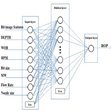
Figure 4 shows the proposed network structure. For network training, the data collected from the field were used to develop a network model. This model computed the forecasted values of ROP based on the input through MATLAB®. The experimental data were random groups, which comprise of 70% training, 15% testing and 15% validation.

In all ANN models, input and outputs were normalized between 0 and 1 to prevent numerical overflows as a result of very large or small weights [22]. The normalization equation is as follows:

yi= xi−xmin

xmax−xmin (8)

where yi refers to the standardized value of xi, xmin refers to xi minimum value, and xmax refers to the maximum value of xi. The ANN model performance was identified by adopting the coefficient of determination (R2) and the Mean Squared Error (MSE) [21-23]. These parameters are shown as below:

𝑀𝑆𝐸 =1

𝑁∑ (𝑦𝑝𝑟𝑑,𝑖− 𝑦𝑒𝑥𝑝,𝑖)

2 𝑁

𝑖=1 (9)

𝑅2_{= 1 −}∑𝑁𝑖=1(𝑦𝑝𝑟𝑑,𝑖−𝑦𝑒𝑥𝑝,𝑖)2

∑𝑁 (𝑦𝑝𝑟𝑑,𝑖−𝑦𝑚)2 𝑖=1

(10)

where 𝑦𝑝𝑟𝑑,𝑖 shows the proposed value by the trained

ANN model, 𝑦𝑒𝑥𝑝,𝑖 represents the experimental value

where N is the number of data, and 𝑦𝑚shows the

average experiment value [24].

TABLE 2. A typical example of second-order surface metrics

Contrast Homogeneity Energy Correlation Entropy IADC

0.1298 0.9685 0.4472 0.9947 0.7579 537

0.1235 0.9677 0.4818 0.9884 0.9130 517

0.0717 0.9795 0.6225 0.9948 0.9544 214

0.0808 0.9840 0.6473 0.9945 0.8960 135

According to the ANN model, the objective function that connects inputs and output can be shown below:

ANN output = Purelin(𝑤2𝑡𝑎𝑛𝑠𝑖𝑔(𝑤1[x(1); x(2); x(3)] + 𝑏1) + 𝑏2)

(11)

where, x (1), x (2) and x (3) refer to the inputs, W1 and W2 refer to the weight and b1 and b2 represent the hidden and output layers bias, respectively. The offset bit records comprise of the offset well drilling operation data. Drilling data comprise of WOB, MW, RPM, bit size, flow rate, nozzle diameter, depth, rotation hour, bit meter, and dull bit grading.

3. RESULTS AND DISCUSSION

An ANN was adopted to the ROP model. The field data were collected using various operational conditions and were used to prepare and test the neural network model [25]. Consequently, the study achieved the best ANN model that appropriates the minimal MSE value for the test set. 1 to 23 neurons were applied in the hidden layer to optimize the network. The study observed that the optimum number of hidden neurons was 18, and the value for MSE was 0.0037, while the R2 was 0.94. This shows that a good agreement between the predicted and experimental data was achieved by the trained model.

The ANN model had taken into account the RPM, bit size, WOB, depth, flow rate, mud weight [10, 26], and image features as its inputs. Therefore, drilling bit selection can result in obtaining the desired ROP through the application of the operational parameters for drilling. The subsequent section provides a description of the bit selection optimization.

Bias

Bias

DEPTH

WOB

RPM

Input layer

Hidden layer

Output layer

Bit size

ROP

Flow Rate Bit image features

MW

Nozzle size

Figure 4. A backward propagation of errors ANN model for

drill bit performance

This optimization was studied to acquire the maximum ROP. Furthermore, Equation (11) was adopted as a GA objective function and the study used the similar number of ANN and GA inputs.

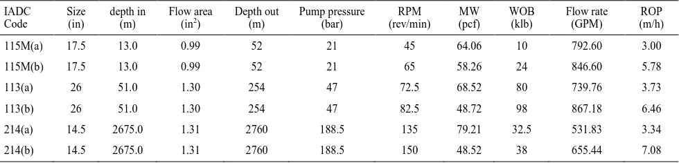
Optimizations for 18 separate drill bits were conducted as examples for the case study. This progress kept the bit size constant and used hydraulic optimization which enabled variation in the parameters including RPM and WOB. Besides, the GA produced the maximum ROP values. This provided the study with the best bit that can be utilized for each hole section [27]. Here, ANN was adopted to obtain the ROP function, the optimum ROP, and related factors including mud flow, RPM, and WOB, throughout the drilling of various hole sections that were probed. As a result, the recommended bit for selection constitutes of one that shows the highest forecasted ROP. The field data prior to optimization (a) and the optimum data proceeding optimization (b) are presented in Table 3. It is worth mentioning that the ANN adopted in this study successfully performed the proper bit selection for new sections, and thus, it can be applied to improve the planning process of a new well. This study obtained the MSE minimum value of 0.0037 and the coefficient of determination (R2) of 0.9473 for the ROP. Figure 5 presents the normalized predicted ROP versus the real ROP. The low error indicates the designed algorithm’s highest performance.

115M, 113 and 214 are milled tooth bits designed for soft formations with low compressive strength and high drillability. After drilling, the cutting structure exhibited no significant wear and bits came out to surface with effective bearings. The bits were in re-run condition and could be considered for another run if needed. Reasons for low ROP are insufficient WOB, RPM and improper flow rate and mud weight. To increase ROP, factors such as WOB, RPM and flow rate can be increased but the limitation for flounder point and maximum flow rate that pump can provide should be considered. Decreasing the mud weight will increase ROP but insufficient mud weight may result in the flow of formation fluids into the borehole or the collapse of borehole.

Figure 5. Predicted ROP versus real ROP

R² = 0.9473

0 0.2 0.4 0.6 0.8 1

0 0.2 0.4 0.6 0.8 1

N

o

rm

al

iz

ed

pr

edi

ct

ed

R

O

P

TABLE 3. Optimum bit and drilling data based on maximum ROP using GA

IADC Code

Size (in)

depth in (m)

Flow area

(in2₎ Depth out _(m) Pump pressure _{(bar) (rev/min)} RPM MW _(pcf) WOB _(klb) Flow rate _{(GPM) (m/h)} ROP

115M(a) 17.5 13.0 0.99 52 21 45 64.06 10 792.60 3.00

115M(b) 17.5 13.0 0.99 52 21 65 58.26 24 846.60 5.78

113(a) 26 51.0 1.30 254 47 72.5 68.52 80 739.76 3.73

113(b) 26 51.0 1.30 254 47 82.5 48.72 98 867.18 6.46

214(a) 14.5 2675.0 1.31 2760 188.5 135 79.21 32.5 531.83 3.34

214(b) 14.5 2675.0 1.31 2760 188.5 150 48.52 38 655.44 7.08

4. CONCLUSION

To extract the bit features in this study, the image processing techniques was used. The artificial neural network was adopted to obtain the mathematical correlation between field drilling data image features and ROP. Moreover, to optimize drilling data, the mathematical equation was adopted as the GA objective function. Based on the ROP equation, this study simulated the drilling process, as well as drilling optimization which leads to the increment of ROP. The optimum bit runs are presented as evaluated by ROP. Consequently, the drilling program was improved through the drilling simulation, and the mathematical model, which represent the ROP, showed good correlation with the bit image features and the real field data. Lastly, the results showed that bit pattern can be inserted in the calculation through a proper bit image processing technique so that each unique bit can be discriminated from other bits. The values of mean square error, 0.0037, and the coefficient of determination (R2), 0.9473, were identified for the rate of penetration model.

5. REFERENCES

1. Fear, M., Meany, N. and Evans, J., "An expert system for drill bit selection", in SPE/IADC Drilling Conference, Society of Petroleum Engineers. (1994).

2. Tools, B.H., "World oil’s 2014 drill bit classifier", (2014). 3. Lyon, R.C., "Planning a bit selection for a deep overthrust well",

in SPE Rocky Mountain Regional Meeting, Society of Petroleum Engineers. (1982).

4. Fear, M., "How to improve rate of penetration in field operations", in SPE/IADC Drilling Conference, Society of Petroleum Engineers. (1996).

5. Burgess, T., "Measuring the wear of milled tooth bits using mwd torque and weight-on-bit", in SPE/IADC Drilling Conference, Society of Petroleum Engineers. (1985).

6. Xu, H., Tochikawa, T. and Hatakeyama, T., "A practical method for modeling bit performance using mud logging data", in SPE/IADC drilling conference. (1997), 127-131.

7. Bilgesu, H., Al-Rashidi, A., Aminian, K. and Ameri, S., "An unconventional approach for drill-bit selection", in SPE Middle East Oil Show, Society of Petroleum Engineers., (2001). 8. Bataee, M., Edalatkhah, S. and Ashena, R., "Comparison

between bit optimization using artificial neural network and other methods base on log analysis applied in shadegan oil field", in International Oil and Gas Conference and Exhibition in China, Society of Petroleum Engineers., (2010).

9. Bilgesu, H., Al-Rashidi, A., Aminian, K. and Ameri, S., "A new approach for drill-bit selection", Journal of Petroleum

Technology, Vol. 52, No. 12, (2000), 27-28.

10. Yιlmaz, S., Demircioglu, C. and Akin, S., "Application of artificial neural networks to optimum bit selection", Computers & Geosciences, Vol. 28, No. 2, (2002), 261-269.

11. Hareland, G., Wu, A., Rashidi, B. and James, J., "A new drilling rate model for tricone bits and its application to predict rock compressive strength", in 44th US Rock Mechanics Symposium and 5th US-Canada Rock Mechanics Symposium, American Rock Mechanics Association., (2010).

12. Rahman, A., Salam, A., Islam, M. and Sarker, P., "An image based approach to compute object distance", International

Journal of Computational Intelligence Systems, Vol. 1, No. 4,

(2008), 304-312.

13. Castejón, M., Alegre, E., Barreiro, J. and Hernández, L., "On-line tool wear monitoring using geometric descriptors from digital images", International Journal of Machine Tools and

Manufacture, Vol. 47, No. 12, (2007), 1847-1853.

14. Haralick, R.M. and Shanmugam, K., "Textural features for image classification", IEEE Transactions on Systems, Man,

and Cybernetics, Vol., No. 6, (1973), 610-621.

15. Shapiro, L. and Haralick, R., "Computer and robot vision",

Reading: Addison-Wesley, Vol. 8, (1992).

16. Dutta, S., Datta, A., Chakladar, N.D., Pal, S., Mukhopadhyay, S. and Sen, R., "Detection of tool condition from the turned surface images using an accurate grey level co-occurrence technique",

Precision Engineering, Vol. 36, No. 3, (2012), 458-466.

17. Clausi, D.A. and Zhao, Y., "Rapid extraction of image texture by co-occurrence using a hybrid data structure", Computers &

Geosciences, Vol. 28, No. 6, (2002), 763-774.

18. Soh, L.-K. and Tsatsoulis, C., "Texture analysis of sar sea ice imagery using gray level co-occurrence matrices", IEEE

Transactions on Geoscience and Remote Sensing, Vol. 37, No.

2, (1999), 780-795.

19. Gebejes, A. and Huertas, R., "Texture characterization based on grey-level co-occurrence matrix", in Proceedings in Conference of Informatics and Management Sciences. (2013).

features and fuzzy svm", Expert Systems with Applications, Vol. 37, No. 10, (2010), 6737-6741.

21. Pradeep, J., Srinivasan, E. and Himavathi, S., "Neural network based recognition system integrating feature extraction and classification for english handwritten", International Journal of

Engineering-Transactions B: Applications, Vol. 25, No. 2,

(2012), 99-106.

22. Khanmohammadi, S., "Neural network sensitivity to inputs and weights and its application to functional identification of robotics manipulators", International Journal of Engineering, Vol. 7, No. 1, 7-12.

23. Sharifzadeh, M. and HosseinAlizadeh, R., "Artificial neural network approach for modeling of mercury adsorption from aqueous solution by sargassum bevanom algae (research note)",

International Journal of Engineering-Transactions B:

Applications, Vol. 28, No. 8, (2015), 1124-1133.

24. Hopfield, J.J., "Artificial neural networks", Circuits and Devices

Magazine, IEEE, Vol. 4, No. 5, (1988), 3-10.

25. Reed, R.D. and Marks, R.J., "Neural smithing: Supervised learning in feedforward artificial neural networks, Mit Press, (1998).

26. Jamshidi, E. and Mostafavi, H., "Soft computation application to optimize drilling bit selection utilizing virtual inteligence and genetic algorithms", in IPTC 2013: International Petroleum Technology Conference., (2013).

27. Arifovic, J. and Gencay, R., "Using genetic algorithms to select architecture of a feedforward artificial neural network", Physica

A: Statistical Mechanics and its Applications, Vol. 289, No. 3,

(2001), 574-594.

Optimum Drill Bit Selection by Using Bit Images and Mathematical Investigation

M. Momenia_{, S. Ridha}a_{, S. J. Hosseini}a_{, X. Liu}a_{, A. Atashnezhad}b_{, S. Ghaheri}a

a _{Department of Petroleum Engineering, Universiti Teknologi PETRONAS, Bandar Seri Iskandar, Perak Darul Ridzuan, Malaysia} b _{Department of Chemical Engineering, Oklahoma State University, Stillwater, USA}

P A P E R I N F O

Paper history:

Received 04 June 2017

Received in revised form 24 August 2017 Accepted 08 September 2017

Keywords: Bit Selection

Artificial Neural Network Image Processing Techniques Genetic Algorithm

Optimum Drilling Operation

ديكچ ه

ا نی سررب روظنم هب هعلاطم ی

دان بلغا اما مهم هناگود لماوع هدی هدش هتفرگ ، هک لماش صوت هی و و هناخراک یگژی اه ی هتم ،تسا باختنا رد هتم بولطم تسا هدش یحارط نکت . کی اه ی وصت شزادرپ ری ارب ی و نتفرگ رظن رد یگژی اه ی هتم هدافتسا .دنا هدش کی زا ر هلداعم یضای زا هک کی بصع هکبش لدم ی

ارب تسا هدش جارختسا ی هتم باختنا یرافح ارب ی تسد هب

م رثکادح ندروآ نازی

ذوفن هتم اهرتماراپ هب هک ی هب هنی ارب ی رافح ی م دوش یم طوبر م هدافتسا

ی ددرگ اپ رد . ،نای هتم رثکادح اب م نازی باختنا ذوفن دوش یم اتن . ی ج ا نی م ناشن هعلاطم ی

وگلا هک دهد ی هتم م ار ی رط زا ناوت قی کی وصت شزادرپ شور ری

هتم ا .داد رارق هبساحم رد بسانم نی ارب ی مطا نانی ا زا هک تسا نی ره

هتم م درف هب رصحنم ی دناوت زا زیامتم هتم اه ی د رگی داقم .دشاب ری اطخ ی م نیگنای رض و عبرم بی یگتسبمه ( R2 ترت هب ) بی 0037 / 0 و 9473 / 0 ارب ی م لدم نازی ذوفن تسد هب دمآ . زا نکت کی اه ی شزادرپ ریوصت ارب ی و جارختسا یگژی اه ی هتم س هبعج .دش هدافتسا های هکبش بصع ی عونصم ی روظنم هب

ر تلاداعم جارختسا یضای

و تیفافش فس هبعج هب ،لدم دی

دبت لی .دش