Detailed Scheduling of Tree-like Pipeline Networks with Multiple Refineries

Please cite this article as: M. Taherkhani, R. Tavakkoli-Moghaddam, M. Seifbarghy, P. Fattahi, Detailed Scheduling of Tree-like Pipeline Networks with Multiple Refineries, International Journal of Engineering (IJE), TRANSACTIONS C: Aspects Vol. 30, No. 12, (December 2017) 1870-1878

International Journal of Engineering

Detailed Scheduling of Tree-like Pipeline Networks with Multiple Refineries

M. Taherkhania_{, R. Tavakkoli-Moghaddam}*b,c_{, M. Seifbarghy}d_{, P. Fattahi}d

a _{Department of Industrial Engineering, Science and Research Branch, Islamic Azad University, Tehran, Iran} b _{School of Industrial Engineering, College of Engineering, University of Tehran, Tehran, Iran}

c _{LCFC, Arts et Métier Paris Tech, Centre de Metz, France}

d _{Department of Industrial Engineering, Faculty of Engineering, Alzahra University, Tehran, Iran}

P A P E R I N F O

Paper history:

Received 29 December 2016 Received in revised form 04 June 2017 Accepted 16 June 2017

Keywords:

Pipeline Scheduling Refinery Supply Chain Multi-product Pipelines

Mixed-integer Linear Programming Demand Uncertainty

A B S T R A C T

In the oil supply chain, the refined petroleum products are transported by various transportation modes, such as rail, road, vessel and pipeline. The latter provides one of the safest and cheapest ways to connect production areas to local markets. This paper addresses the operational scheduling of a multi-product tree-like pipeline connecting several refineries to multiple distribution centers under demand uncertainty. A new deterministic mixed-integer linear programming (MILP) model is first presented, and then a two-stage stochastic model is proposed. The aim of this model is to meet depot requirements at the minimum total cost including pumping and stoppages costs. The efficiency and utility of the proposed model is shown by two numerical examples, which one of them uses the industrial and real data.

doi: 10.5829/ije.2017.30.12c.08

1. INTRODUCTION1

Nowadays, operations of a supply chain and logistics are among the most important activities in companies [1]. Transportation is an important supply chain driver because products are rarely produced and consumed in the same location [2]. Multi-product pipeline conveying a variety of petroleum products are the most common means of transportation in the oil industry to transfer the products from refineries to depots. Transportation planning of petroleum products via pipelines is one of the most challenging management problems in the oil industry and can increase the annual profit in several millions of dollars. Multi-product pipelines stay full with product at any time. Consequently when some products enter inside a pipeline, the same volume should leave that line. Some product sequences are forbidden inside the pipelines; for instance, gas and oil should never be adjacent to gasoline. Pipeline structures vary from straight to treelike and mesh structures. This

*Corresponding Author’s Email: [email protected] (R. Tavakkoli-Moghaddam)

paper is concerned with a tree-like pipeline system that must distribute a number of petroleum products from multiple refineries to several depots. Finding the best sequence of product injections at refineries, which product removals at depots and the length of pumping operations for multi-product ducts to satisfy product demands requested by distribution centers on time at the minimum total cost, is the most important element of pipeline scheduling problem. Several operational constraints should also be considered. These include keeping the inventory level of depots at the acceptable range and maintaining the flow rate in different segments at the feasible range.

structure including a single refinery and single distribution center Relvas et al. [3] and Cafaro and Cerda [4], or single refinery with multiple destinations Hane and Ratliff [5] and Rejowski and pinto [6] and Cafaro and Cerda [7] Mostafaei and Ghaffari Hadigheh [8], or multiple refineries and distribution centers, Cafaro and Cerda [9] Mostafaei et al. [10, 11] to more complex cases with branching configuration Castro and Grossman [12] and Cafaro and Cerda [13] and Herran et al. [14] Desouza Filho et al. [15] and Boschetto et al. [16]and Mostafaei et al. [17] and bidirectional pipeline systems connecting a refinery to a harbor [18, 19].

All paper mentioned above have focused on the aggregate planning providing the optimal sequence of batch injections during a known planning horizon. None of them focuses on determining the optimal sequences of stripping operations at receiving terminals to generate a detailed delivery schedule and to get savings in pump operating and maintenance costs. Cafaro et al. [20, 21] used hierarchical decomposition approaches for detailed scheduling of straight of pipeline networks. Mostafaei et al. [22-25]developed monolithic MILP frameworks for detailed scheduling of straights pipeline that achieve better solution with respect to decomposition approaches.

Mostafaei et al. [26] presented an MILP model for detailed scheduling of tree-like pipeline connecting a single refinery to multiple depots. The model is based on a continuous time representation in both volume and time scales. Given product demands at depots, the proposed model determines both input and output operations of the pipeline in a single step. However, the model can only be applied to tree-like pipeline with a single refinery and with deterministic product demands at depots. The contribution of this paper is as follows. Firstly, a generalization of the model presented by Mostafaei et al. [26] from a unique refinery at the origin of the pipeline to multiple refineries with dual purpose stations is developed. Secondly, contrarily to the previous studies considering product demands at pipeline depot as deterministic data, the proposed

approach uses stochastic datum for a product requirement.

The rest of this paper is organized as follows. Section 2 gives a concise description of the problem under study. Section 3 presents the model assumptions. Section 4 presents the deterministic MILP model for a tree-like scheduling problem. Section 5 proposes a stochastic counterpart of the MILP model. Section 6 gives two case studies to show the validation of the proposed model. The paper ends with the conclusions.

2. PROBLEM STATEMENT

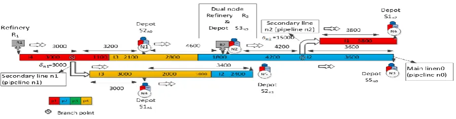
This paper addresses the scheduling of a tree-like pipeline network with a mainline (pipeline n0), several secondary lines, multiple refineries, depots and dual purpose stations. Figure 1 depicts a tree-like pipeline network with two refineries, two secondary lines (i.e., pipeline n1 and n2). A dual purpose node composes of refinery R2 and depot N2. The refineries inject refined petroleum products into the pipeline while depots receive them. The dual purpose station performs both injecting and receiving operations. We use terms “secondary line” or “branching line” for pipelines that are emerged from the mainline. In Figure 1, the first secondary line leaves the mainline at point 3000 m3 while the second one branches at point 15000 m3. The volume of a product is regarded as a batch, in which each batch only conveys one product and can be at most adjacent to two products. For example, in Figure 1, batch I3 in the mainline (i.e., yellow rectangle) conveys product P3 and touches two batch I2 and I4 conveying products P2 and P1, respectively. Note that each pipeline is divided into segments, in which each segment ends with a depot or branch point. The mainline composes of five segments, in which the segments of the pipeline network and their volume are specified by left and right arrows.

The existence batches inside the pipeline n at the start time of the time horizon are given by old batches (Inold).

The set of old batches of pipeline n0, n1 and n2 is

In0old= {I2 , I3, I4}, In1old= {I2 , I3} and In2old= {I1 }, respectively. The set of new batches, which enter in to pipeline n during the scheduling horizon, is new batches (Innew). In this paper, the number of new batches to be injected into the mainline is known beforehand. For instance, if we assume that two new batches I5 and I6 are injected into the mainline of Figure 1 during the planning horizon, we have In0new{I5 , I6}, In1new{I4, I5 , I6} and In2new{I2, I3 , I4, I5 , I6}. Set In= Innew∪Inold is the set of batches to move in pipeline n during planning horizon. The set of batches that can be injected from refinery r into mainline during planning horizon is given by Ir.

In Figure 1, refinery R1 can only inject batches I4, I5 and I6 and so 𝐼𝑟1= {I4, I5 , I6} whereas refinery R2 can increase the size of batch I2, I3,…, and so 𝐼𝑟2=

{I2 , I3, I4, I5 , I6}. The set 𝐼𝑛𝑆 is set of batches that can be received by depot 𝑠𝑛 (depot 𝑠 on pipeline 𝑛). For example, in Figure 1, depot 𝑠1𝑛0= N1 can only receive product from batch I3 and batches I4, I5 and I6 that will pass from the output facility of this depot in the future; however, batch I2 can never be transferred to depot N1, and so we have 𝐼𝑛0𝑠1= {𝐼3 , 𝐼4, 𝐼5 , 𝐼6}.

3. MATHEMATICAL MODEL

To develop a mathematical tool based on an MILP framework, the following assumptions are to be considered.

 A tree-like pipeline with a single mainline and several branch lines only emerged from the mainline is considered. Flow in all pipelines (mainline ant its branches) is unidirectional.

 Several refineries can be considered on the mainline; however, there is no refinery on branch point and branch line.

 All pipeline segment stay full of product at any time.

 Sequence, content and coordinate of old batches in each segment are known.

 Maximum and minimum flow rates in pipeline segments are given.

 Because of vast product contamination, some products can never touch each other inside the pipeline.

 At each pumping operation, an active depot can receive material from a single batch.

 Demand for each product is random variable (ξp,s,n) with a continuous uniform distribution (ξp,s,n∩ [ap,s,n, bp,s,n]).

This section presents the proposed MILP formulation for the short term scheduling of a tree-like

pipeline system with several refineries and depots. The base model is the mathematical formulation of Mostafaei et al. [26] with the following differences: (1) our approach considers a tree-like pipeline network with several refineries and even dual purpose nodes whereas their approach deals with a single refinery at the origin of the mainline and (2) our approach considers product demands at depots as stochastic variables whereas their approach treats product demand as a deterministic datum. The sets, parameters and continuous and binary variables are all defined from Tables 1 to 3.

3. 1. Sequencing Pumping Runs The start time of pumping run k will be equal to the start time of pumping run k − 1 plus the length of run k − 1.

, 2

1 1

ST_k ST_k L_k  k (1)

3. 2. Location of Batch 𝑖 ∈ 𝐼 in Mainline and Branch Lines Continuous variable 𝐿𝑃𝑉𝑖,𝑘,𝑛 is the upper coordination of batch 𝑖, which is equal to the total volume between the origin of pipeline 𝑛 to the end of batch 𝑖. In Figure 2, the upper coordinate of batch I2 in the mainline is 5000+2000=7000 m3. Note that

𝐿𝑃𝑉𝑖,𝑘,𝑛− 𝑆𝑃𝑉𝑖,𝑘,𝑛 is the lower coordinate of batch 𝑖.

, , ,

, , _' ', ,

LPV_{i k n} SPV_{i k n} i I_n k K n N i i



    

 (2)

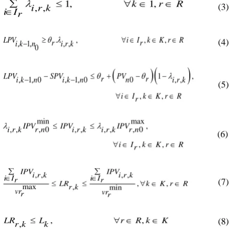
3. 3. Main line feeding operation By Equation (3), only a single batch 𝑖 ∈ 𝐼𝑟 can be injected from refinery 𝑟 during each pumping operation and the coordinates of this batch satisfy Equations (4) and (5). The volume injected from refinery r will always be between [𝐼𝑃𝑉𝑟,𝑛0min, 𝐼𝑃𝑉𝑟,𝑛0max].

TABLE 1. List of sets and indices

Sets Description

𝐾 Set of pumping operations indexed by 𝑘, 𝑘 = 0, 1, … , |𝐾|

𝑁 Set of pipelines indexed by 𝑛, 𝑛′_{, 𝑛′′ = 0, 1, … , |𝑁|}

𝑅 Set of refineries indexed by 𝑟, 𝑟′ = 1, … , |𝑅|

𝐼 Set of all product batches indexed by 𝑖, 𝑖′_{, 𝑗 = 1, … , |𝐼|}

𝑆𝑛 Set of depots on pipeline 𝑛 indexed by 𝑠, 𝑠′, 𝑠′′

𝐼𝑟 Set of batches that can receive material from refinery

𝑟(𝐼𝑛

⊂ 𝐼)

𝐼𝑛𝑜𝑙𝑑 Set of old batches inside pipeline 𝑛(𝐼𝑛𝑜𝑙𝑑⊂ 𝐼)

𝐼𝑛𝑛𝑒𝑤 Set of new batches of pipeline 𝑛(𝐼𝑛𝑛𝑒𝑤⊂ 𝐼)

𝐼𝑛 Set of batches to be moved in pipeline 𝑛 (𝐼𝑛= 𝐼𝑛𝑜𝑙𝑑∪ 𝐼𝑛𝑜𝑙𝑑)

𝐼𝑛𝑆 Set of batches that can be diverted into depot 𝑠𝑛(𝐼𝑛𝑠⊂ 𝐼)

TABLE 2. List of parameters

Parameters Description

ℎmax The length of schedule horizon (h)

𝐶𝑃𝑝,𝑟 Pumping cost of product 𝑝 at refinery 𝑟($/m3)

𝐶𝐵𝑝,𝑠,𝑛 Backorder cost of product _($/m3₎ 𝑝 in the depot 𝑠𝑛𝑡

𝑣𝑟𝑟min/ 𝑣𝑟𝑟max Min / max injection rate at refinery 𝑟 (m3/h)

𝐼𝑃𝑉𝑟max/𝐼𝑃𝑉𝑟max Min / max batch injected size in mainline in each _{run (m}3

)

𝐼𝑅𝑉𝑛min/𝐼𝑅𝑉𝑛max

Min / max batch size transferred to branch line

𝑛 in each run (m3₎

𝐷𝑃𝑉𝑠,𝑛max/𝐷𝑃𝑉𝑠,𝑛min Min / max batch size transferred to depot _{each run (m}3₎ 𝑠𝑛 in

𝑣𝑠𝑠,𝑛max/𝑣𝑠𝑠,𝑛min Min/max flow rate in segment 𝑠𝑛

𝜃𝑟 Volumetric coordination of refinery _{origin of mainline (m}3 𝑟 from the

)

𝜎𝑛 Volumetric coordination of secondary line _{from the origin of mainline (m}3 𝑛

)

𝜏𝑠,𝑛 Volumetric coordinate of depot _{origin of pipeline 𝑛 (m}3₎ 𝑠𝑛 from the

𝑃𝑉𝑛 Volume of pipeline 𝑛 (m3)

𝑟𝑒𝑓𝑡𝑝,𝑟 Inventory of product 𝑝 in refinery 𝑟 during planning horizon (m3)

𝑇𝑜𝑢𝑐ℎ𝑝,𝑝′ Boolean matrix of possible sequences between products p and 𝑝′ _(m3)

𝐷𝑒𝑚𝑎𝑛𝑑𝑠,𝑛,𝑝 Demand of product 𝑝 of depot 𝑠𝑛 (m3)

𝐼𝑆𝑃𝑉𝑖,𝑛 Size of old batch _(m3₎ 𝑖in the pipeline 𝑛 at time 𝑠𝑡𝑓

𝑉𝑆𝐸𝐺𝑠,𝑛 The volume of segment 𝑠𝑛 (m3)

TABLE 3. List of variables Description Continuous

Variables

Start time of composite pumping run 𝑘 (h)

𝑆𝑇𝑘

Activity length of refinery 𝑟 though composite pumping run 𝑘 (h)

𝐿𝑅𝑟,𝑘

Length of composite pumping run 𝑘 (h)

𝐿𝑘

Unsatisfied demand of product 𝑝 in depot 𝑠𝑛 (m3)

𝐵𝑎𝑐𝑘𝑝,𝑠,𝑛

Size of batch 𝑖 ∈ 𝐼𝑟 injected into the mainline from the refinery 𝑟 during composite pumping run 𝑘 (m3₎

𝐼𝑃𝑉𝑖,𝑟,𝐾

Size of batch 𝑖 ∈ 𝐼𝑟 conveying product 𝑝 injected from the refinery 𝑟 to mainline during composite pumping run 𝑘 (m3_).

𝑃𝑃𝑉𝑖,𝑝,𝑟,𝑘

Volume of batch 𝑖 ∈ 𝐼𝑛 transferred to branching line

𝑛 during run 𝑘 (m3₎

𝐼𝑅𝑉𝑖,𝑘,𝑛

Size of batch 𝑖 ∈ 𝐼𝑛𝑠 diverted to depot 𝑠𝑛 during composite pumping run 𝑘 (m3₎

𝐷𝑃𝑉𝑖,𝑠,𝑘,𝑛

Size of batch 𝑖 ∈ 𝐼𝑛𝑠 covering product 𝑝 diverted to depot 𝑠𝑛 during run 𝑘 (m3)

𝑃𝐷𝑃𝑉𝑖,𝑝,𝑠,𝑘,𝑛

Upper coordinate of batch 𝑖 ∈ 𝐼𝑛at the end of pumping run 𝑘 (m3)

𝐿𝑃𝑉𝑖,𝑘,𝑛

Size of batch 𝑖 ∈ 𝐼𝑛at the end of pumping run 𝑘 (m3)

𝑆𝑃𝑉𝑖,𝑘,𝑛

stopped volume of segment 𝑠𝑛at the end of pumping run k(m3₎

𝑆𝑉𝑠,𝑘,𝑛

Binary variables

1 if batch 𝑖 ∈ 𝐼𝑟 is injected from refinery 𝑟 to the main line during run 𝑘

𝜆𝑖,𝑟,𝑘

1 if secondary line 𝑛 receives batch 𝑖 during run 𝑘 𝑢𝑖,𝑘,𝑛

1 if batch 𝑖 ∈ 𝐼𝑛𝑠 is diverted to depot 𝑠𝑛 during run 𝑘

𝑥𝑖,𝑠,𝑘,𝑛

1 if batch 𝑖 transports product 𝑝 𝑦𝑖,𝑝

1 if segment 𝑠𝑛is active during run k

𝑒𝑠,𝑘,𝑛

1 if some portion of batch 𝑖 exists in branching line 𝑛 𝑧𝑖,𝑛

The activity duration of all active refineries is of the same value and determined the length of a pumping operation, as imposed by Equation (8).

1, 1,

, , k r R

i r k

i Ir      (3)

. , , ,

, 1,₀ , ,

LPV_{i k n}  _{r i r k}  i I_r kK rR ₍₄₎









, 1, 0 , 1, 0 , ,

, ,

LPV_{i k n} SPV_{i k n r} PV_{n r i r k}

i I_r k K r R

  

    

 

   

(5)

min max

,

, 0 , 0

, , , , , ,

, ,

IPV_{r n} IPV IPV_{r n}

i r k i r k i r k

i I_r k K r R

  

    (6)

, , , ,

, ,

max , min

IPV_{i r k} IPV_{i r k}

i I_r i I_r

LR_{r k} k K r R

vrr vrr

 

 _{ }  _{   (7)}

, ,

,

LR_{r k} L_k  r R kK (8)

3. 4. Batch Feature Constraints It should be noted that each batch 𝑖 ∈ 𝐼𝑛 contains only one product 𝑝, Equation

(9). If batch 𝑖 contains product p then the size of the continuous variable 𝑃𝑃𝑉𝑖,𝑝,𝑟,𝑘 will be equal to 𝐼𝑃𝑉𝑖,𝑟,𝑘;

otherwise, it will be equal to zero, Equations (10) and (11). The volume of product p added to the main line from refinery r during the scheduling should be equal or smaller than 𝑟𝑒𝑓𝑡𝑟,𝑝.

1, ,

y_{i p} i I

, , , , , , , ,

PPV_{i p r k} IPV_{i r k} i I_r p P r R

p P      (10)

1

max

. ₀ . _, , , ,

, , ,

k

PPV_{i p r k} K IPV_n y_{i p} i I_r p P r R

     



PPV_{i p r k} reft_{r p} r R p P i I

k K _r     (12)

3. 5. Operation of Unloading the Main Line and Branch Lines The binary variable 𝑥𝑖,𝑠,𝑘,𝑛 is equal to 1 if batch 𝑖 ∈ 𝐼𝑠𝑛 is sent to depot 𝑠𝑛 during the execution of pumping 𝑘. A portion of batch 𝑖 ∈ 𝐼𝑛 can be received by depot 𝑠𝑛only if the coordinates of the batch satisfy Equations (13) and (14). When 𝑥𝑖,𝑠,𝑘,𝑛=

1, depot 𝑠𝑛 will receive a positive portion of batch 𝑖 ∈

𝐼𝑠𝑛, as imposed by Equation (15). If batch 𝑖 ∈ 𝐼𝑠𝑛 contains product p the value of the continuous variable

𝑃𝐷𝑃𝑉𝑖,𝑝,𝑠,𝑘,𝑛will be equal to 𝐷𝑃𝑉𝑖,𝑠,𝑘,𝑛; otherwise, it is equal to zero, as imposed by Equations (16) and (17).

. ,

,

, 1, , , ,

, , ,

LPV_{i k n s n}x_{i s k n} n

i I_s k K s S n N



 

     (13)









, ,

, , , , , , ,

, , ,

LPV_{i k n} SPV_{i k n s n} PV_{n s n} x_{i s k n} n

i I_s k K s S_n n N

            (14) min max , , , , , , , , , , , , , , ,

x_{i s k n}DPV_{s n} DPV_{i s k n} x_{i s k n}DPV_{s n}

n

i I_s k K s S_n n N

       (15) , , , , , , , , , , ,

PDPV_{i p s k n} DPV_{i s k n} p

n

i I_s k K s S_n n N

       (16) max . , , , , , , , , ,

PDPV_{i p s k n} K DPV_{s n} y_{i p} k

n

i I_s s S_n n N

 

   

(17)

3. 6. Branch Lines Feeding Operation The binary variable 𝑢𝑖,𝑘,𝑛= 1 shows that batch 𝑖 ∈ 𝐼𝑛 in pumping k is transferring to the branch line 𝑛. A portion of batch 𝑖 in mainline can be received by branch line

𝑛 only if the coordinates of the batch satisfy Equations (18) and (19). By Equation, (20), when 𝑢𝑖,𝑘,𝑛= 1, branch line n will receive a proportion of batch 𝑖 ∈ 𝐼𝑛.

,

, 1, 0 , ,

, , , 0

LPV_{i k n n}u_{i k n}

i I_n k K n N n n

  

     (18)

( ₀ )(1 ),

, , 0 , , 0 , ,

, , , 0

LPV_{i k n} SPV_{i k n n} PV_{n n} u_{i k n}

i I_n k K n N n n

 

    

     (19)

min max

,

, , , , , ,

, , , 0

IRV_n u_{i k n} IRV_{i k n} IRV_n u_{i k n}

i I_n k K n N n n

 

    

(20)

3. 7. Mass Balance Constraints The continuous variable 𝑆𝑃𝑉𝑖,𝑘,𝑛 is the volume of batch 𝑖 at the end of pumping k in pipeline n. Volume of batch 𝑖 at the end of pumping k in the main line and branch lines is shown by Equations (21) and (22).

, , 0 , 1, 0 , ,

,

, , , 0 , ,

0

, , 1

0

SPV_{i k n} SPV_{i k n} IPV_{i r k}

r R

DPV_{i s k n} IRV_{i k n}

s S_n n SP

i I_n k K k

  _             (21) ,

, , , 1, , , , , ,

, , , ₀

SPV_{i k n} SPV_{i k n} IRV_{i k n} DPV_{i s k n} s Sn

i I_n k K n N n n

  _         (22)

In the main line and branch lines, the injected volume is always equal to the output volume, Equations (23) and (24).

,

, , , , ,

, , 0

IRV_{i k n} DPV_{i s k n}

i I_n s S i I_{n n}

k K n N n n

   

  

   

(23)

, , , , , 0

0 0

, , ,

, 0

IPV_{i r k} DPV_{i s k n}

i I r Rr s S_n i I_n

IRV_{i k n} k K

n N n n i In

                 (24)

3. 8. Forbidden Sequences For quality reasons some products should not touch together inside the pipeline. For example in real pipelines, a batch of gasoline (premium, regular, etc.) should never be adjacent to a batch of gas oil. If 𝑇𝑜𝑢𝑐ℎ_𝑝,𝑝′ = 1, product

𝑝 and 𝑝′ can touch together inside the pipeline, otherwise their sequence is forbidden. This restriction are controlled by:

1,

, 1, ,

, ,

y_{i p} y_{i p} Touch_{p p}

i I p p P

 _{ }  _



   (25)

 

3,

, , , , , ,

, , , , 0

z_{i n} z_{i n} z_{j n} y_{i p} y_{i p} Touch_{p p}

new

i I_n i I_n i i p p P n n



 _    _{ } _

  

     

where 𝑧𝑖,𝑛 is a binary variable denoting the existence of batch 𝑖′ ∈ 𝐼𝑛 in secondary line 𝑛 and satisfies the following eq 𝑧𝑖,𝑛≤ ∑ 𝑢𝑘 𝑖,𝑘,𝑛≤ |𝐾|𝑧𝑖,𝑛, ∀𝑖 ∈ 𝐼𝑛𝑛𝑒𝑤, 𝑛 ∈

𝑁, , 𝑛 ≠ 𝑛0.

3. 9. Constraints Satisfied Demand In a deterministic mode, the demand of depots is the known parameter 𝐷𝑒𝑚𝑎𝑛𝑑𝑠,𝑛,,𝑝 and should be satisfied on time. This unsatisfied demand (𝐵𝑎𝑐𝑘𝑠,𝑛,𝑝) will result in backorder costs.

,

, , , ,

, , , ,

, , ,

PDPV_{i p s k n} Demand_{s n p} Back_{s n p} s

k K i In

p P s S_n n N k K

   

 

    

(27)

3. 10. Identifying Active and Ideal Segments The binary variable 𝑒𝑠,𝑘,𝑛 determines the status (active or idle) of segment 𝑠 ∈ 𝑠𝑛during pumping run 𝑘 and its value satisfy the following equations:

0, , 0,

e_{s k n} n N

s Sn    (28)

, , 1, 1, , 0 1

e k K

i r k s k n

i I_r     (29)

, , , , , ,

( ), ,

x e

i s k n s k n s

i In

s last S_n k K n N

 



   

(30)

1, 0 , 0

1, 0 , 0

, , , , 0

,

, , 1, ,

, 0

i I

r r

s n s n

i I

r r

s n s n

e i r k s k n

e i r k s k n

s S_n k K

                      _{ }    (31) 0

, 0 1, 0 0

, , , 0 , , 0

1 _{, , , 0 , ,} ,

, 0

s i In

s _{i I}

i In s n r s n r

x_{i s k n} e_{s k n}

x_{i s k n i r k}

s S_n k K

                     (32) , , , , ,

0, , ( )

e_{s k n} u_{i k n}

i In

n n k K s _{first Sn}

       (33) , , , , , , , ,

x_{i s k n} e_{s k n} s

i In

k K s S_n n N

 



   

(34)

,

, , 0 , ,

0, ,

e_{s k n} u_{i k n}

i In

n n k K s S

 



   

(35)

3. 11. Flow Rate Constraints is Mainline and Branch Lines Segments During any pumping run 𝑘 ∈ 𝐾, the flow rate at each active segment 𝑠 ∈ 𝑠𝑛 should belong to feasible range [𝑣𝑠𝑠,𝑛min, 𝑣𝑠𝑠,𝑛max]. Equations (36) and (37) control the flow rate limitation on mainline and its branch, respectively.

min

, , 0 , , , 0

0 '

max

, , , , ₀

, 0 ,₀

(1 )

,

, 0

k S_n s k n _s i s k n

s s i I_n

i k n i r k k S_n

i I i I

s n n n r s r

L vs e DPV

IPV IRV L vs

s S_n k K

                          (36) min max , , , , , '

(1 ) ,

, , , 0

k S_n s k n _s i s k n k S_n s s i I_n

L vs e DPV L vs

s S_n k K n N n n

              (37)

3. 12. Stoppages Volume Continuous variable

𝑆𝑉𝑠,𝑘,𝑛is the stoppage volume of segment 𝑠 of pipeline

𝑛 during pumping run 𝑘. If 𝑒𝑠,𝑘−1,𝑛= 1 and 𝑒𝑠,𝑘,𝑛 = 0, the stopped volume of the segment 𝑠𝑛 will be the volume of segment 𝑠𝑛 (𝑉𝑆𝐸𝐺𝑠,𝑛), otherwise it will be zero.

, , , ( , 1, , , ),

, ,

s k n s k n s k n

SV VSEG_{s n} e e

k K n N s _Sn



 

    (38)

3. 13. Problem Objective Function The problem purpose is to minimize the total tree-like pipeline operating costs including (a) the product pumping cost, (b) backorder demand and (c) pipeline stoppage cost.

min _, . _{, , ,}

. .

, , , , , ,

z cp_{p r}PIV_{i r p k}

r i p k

cb_{s n p}Back_{s n p} cs SV_{s k n}

n s p nk s

   

 

     

4. STOCHASTIC COUNTERPART

Now in this section, we extend the model for the case demand for each product is random variable 𝜉𝑝,𝑠,𝑛∩

[𝑎𝑝,𝑠,𝑛, 𝑏𝑝,𝑠,𝑛]. The objective function can be written as a two-stage stochastic model shown below:

Min 𝑧−s= ∑𝑘∈𝐾∑𝑖∈𝐼𝑟∑𝑝∈𝑃∑𝑟∈𝑅𝑐𝑝𝑝,𝑟. 𝑃𝐼𝑉𝑖,𝑟,𝑝,𝑘+

+ ∑ ∑ ∑ 𝑐𝑠. 𝑆𝑉𝑛 𝑘 𝑠 𝑠,𝑘,𝑛+ ∑ ∑ ∑ 𝐸 (𝑄(𝜆𝑝 𝑠 𝑛 𝑝,𝑠,𝑛, 𝜉𝑝,𝑠,𝑛))

s.t.

Equations (1) − (26), (28) − (38)

where, 𝑄(𝜆𝑝,𝑠,𝑛, 𝜉𝑝,𝑠,𝑛) is the optimal cost if depot 𝑠𝑛 receives 𝜆𝑝,𝑠,𝑛 = ∑𝑘∈𝐾∑𝑖∈𝐼𝑃𝐷𝑃𝑉𝑖,𝑝,𝑠,𝑘,𝑛 units of product 𝑝 while demand is random variable 𝜉𝑝,𝑠,𝑛∩

𝑄(𝜆𝑝,𝑠,𝑛, 𝜉𝑝,𝑠,𝑛) = min ∑ 𝑐𝑏𝑝 𝑝𝐵𝑅𝑝,𝜉𝑝

s.t.

𝐵𝑎𝑐𝑘𝑠,𝑛,𝑝≤ 𝜉𝑝,𝑠,𝑛

𝐵𝑎𝑐𝑘𝑠,𝑛,𝑝≥ 𝜉𝑝,𝑠,𝑛− 𝜆𝑝,𝑠,𝑛

Cleary the optimal value for 𝑄(𝜆𝑝,𝑠,𝑛, 𝜉𝑝,𝑠,𝑛) is max {𝜉𝑝,𝑠,𝑛− 𝜆𝑝,𝑠,𝑛, 0}.

Since 𝜉𝑝,𝑠,𝑛∩ [𝑎𝑝,𝑠,𝑛, 𝑏𝑝,𝑠,𝑛], there are three cases:

𝐸 (𝑄(𝜆𝑝, 𝜉𝑝)) =

{

(𝑎𝑝,𝑠,𝑛−𝜆𝑝,𝑠,𝑛)2

2(𝑏𝑝,𝑠,𝑛−𝑎𝑝,𝑠,𝑛), (𝑏𝑝,𝑠,𝑛−𝜆𝑝,𝑠,𝑛)2

2(𝑏𝑝,𝑠,𝑛−𝑎𝑝,𝑠,𝑛)

0, ,

𝜆𝑝,𝑠,𝑛≤ 𝑎𝑝,𝑠,𝑛

𝑎𝑝,𝑠,𝑛≤ 𝜆𝑝,𝑠,𝑛≤ 𝑏𝑝,𝑠,𝑛

𝑏𝑝,𝑠,𝑛≤ 𝜆𝑝,𝑠,𝑛

So, the objective function is given by:

Min 𝑧−s=

{

∑𝑘∈𝐾∑𝑖∈𝐼𝑟∑𝑝∈𝑃∑𝑟∈𝑅𝑐𝑝𝑝,𝑟. 𝑃𝐼𝑉𝑖,𝑟,𝑝,𝑘+ ∑ ∑ ∑ 𝑐𝑠. 𝑆𝑉𝑛 𝑘 𝑠 𝑠,𝑘,𝑛+ ∑ ∑ ∑ ∑ ∑ 𝑐𝑏𝑝,𝑠,𝑛

(𝑎𝑝,𝑠,𝑛−𝑃𝐷𝑃𝑉_{𝑖,𝑝,𝑠,𝑘,𝑛})2

2(𝑏𝑝,𝑠,𝑛−𝑎𝑝,𝑠,𝑛)

𝑛 𝑠 𝑝∈𝑃 𝑖∈𝐼

𝑘∈𝐾 ,

∑𝑘∈𝐾∑𝑖∈𝐼𝑟∑𝑝∈𝑃∑𝑟∈𝑅𝑐𝑝𝑝,𝑟. 𝑃𝐼𝑉𝑖,𝑟,𝑝,𝑘+ ∑ ∑ ∑ 𝑐𝑠. 𝑆𝑉𝑛 𝑘 𝑠 𝑠,𝑘,𝑛+ ∑ ∑ ∑ ∑ ∑ 𝑐𝑏𝑝,𝑠,𝑛

(𝑏𝑝,𝑠,𝑛−𝑃𝐷𝑃𝑉_{𝑖,𝑝,𝑠,𝑘,𝑛})2

2(𝑏𝑝,𝑠,𝑛−𝑎𝑝,𝑠,𝑛)

𝑛 𝑠 𝑝∈𝑃 𝑖∈𝐼

𝑘∈𝐾 ,

∑𝑘∈𝐾∑𝑖∈𝐼𝑟∑𝑝∈𝑃∑𝑟∈𝑅𝑐𝑝𝑝,𝑟. 𝑃𝐼𝑉𝑖,𝑟,𝑝,𝑘+ ∑ ∑ ∑ 𝑐𝑠. 𝑆𝑉𝑛 𝑘 𝑠 𝑠,𝑘,𝑛,

Case 1

Case 2

Case 3

Cases 1 and 3 are not economical ones since Case 1 seeks for the optimal cost in a lower level demand and Case 3 just leads to an infeasible solution in most cases. So, Case 2 is being tackled in the two-stage stochastic model. Note that the stochastic counterpart of the deterministic model is a mixed-integer quadratic programming (MIQP) model.

5. RESULTS AND DISCUSSION

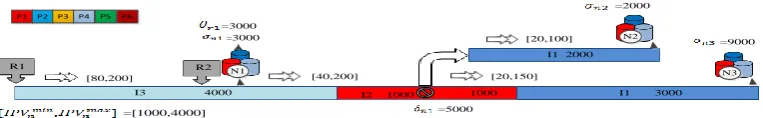
In this section, two case studies are solved. The first one is a simple structure and uses the deterministic data for the demand while the second one uses the industrial data and demands are random variables with a continuous uniform. All MILP models are implemented on GAMS 24.1.2 / CPLEX using an Intel i7-4790K (4.0 GHz) processor and 8 GB of RAM. Note that the stochastic counterpart of the proposed deterministic model was solved using GAMS 24.1.2 / BARON. 5. 1. Case Study 1 This example, which is a small tree network with deterministic demands, deals with a tree-like pipeline network for transporting six products from two refineries to three depots and is a variant of a case study introduced recently by Mostafaei et al. [26]. Note that depot N1isconsidered as a dual purpose node. Maximum and minimum batch sizes injected/diverted to each pipeline/depot though any pumping run, depot and

branch point volume coordinates and flow rate range at segments, are shown in Figure 2. Product inventories and pumping cost at refinery and product demands for next 5 days at depots are given in Table 4. Unit backorder cost is $200/m3 and unit stoppage cost is $1/ m3.

Table 5 shows computational results of Case study 1. Compared to the previous work [26], the proposed approach finds the optimal solution in a lower CPU time due to a lower number of pumping operations, having a major impact on the problem size in term of the number of variables and equations.

5. 2. Case Study 2 This example is a real-world problem of the oil pipeline industry, which a variant of the real world case study introduced by Mostafaei et al. [24] that incorporates a dual purpose node on the mainline. The pipeline structure is depicted in Figure 1. The pump rate at refineries should be kept between 300 and 800 m3/h. The length of planning horizon is

ℎmax= 192 h. The maximum injection volume into each pipeline is 15000 m3 while the minimum one is 500 m3. The minimum delivery to each depot is also 500 m3. The inventory of products at refinery and also pumping cost of each product are all listed in Table 6. Unit flow stoppage cost is 1.0 $/m3. Demand for each product at pipeline depots is random variable (𝜉𝑝,𝑠,𝑛) with a continuous uniform distribution in [3000; 10000], given in m3.

N1

N2

N3

I1 2000

I1 3000

I2 1000 1000

I3 4000

R1 R2

[80,200] [40,200]

[20,100]

[20,150] =3000

=5000

=2000

=9000 =3000

=[1000,4000]

=[1000,4000]

Branch point

Flow rate rang

P1 P2 P3 P4 P5 P6

TABLE 4. Related data for Example 1

Inventory (m3_{) umping cost ($/m}3_{) Demand (m}3₎

P R1 R2 R1 R2 N1 N2 N3

P1 9000 12 0 2000 1000 3000

P2 - 12000 5.5 4 0 2000 2000

P3 10000 10 0 3000 0 0

P4 5000 12.5 0 2000 0 3000

P5 8000 8 0 2000 0 0

P6 5000 7500 5.5 5 0 0 0

TABLE 5. Computational results of Case 1

Case #Pump runs CPU (s) Con. Var Bin. Var Eqs. Back order (%) Pump cost ($) Stop cost ($) Obj. Fun. ($)

Our approach 6 24 2047 318 3884 0 182000 6000 188000

Mostafaei et al. [26] 10 141 2597 399 4486 0 248500 8000 256500

TABLE 6. Inventory and pumping cost

Inventory (m3) Pumping cost ($/m3)

P R1 R2 R1 R2

P1 36000 - 8 -

P2 25000 18000 7.5 6

P3 10000 18000 8 5

P4 42000 - 7 -

Other data related to this example (i.e., the size of old batches, the coordinate of refineries, depots and branch points, the volume of segments and flow rate limitation) can be found in Figure 1. To solve the problem formulation, we set the number of new batches to be injected into the mainline equal to 4 (i.e., 𝐼𝑛𝑛𝑒𝑤=

{I5, I6, I7, I8}). The optimal solution includes nine pumping operations and is found in 2730 s of CPU. At the optimum, the new batches I5, I6, I7 and I8 convey products P3, P2, P4 and P2, respectively. Such product sequences inputted in the pipeline lead to an optimal cost of $534233.

6. CONCLUSION

This paper has presented a new optimization framework for the detailed scheduling of tree-like pipelines featuring multiple refineries and depots. The proposed approach has overcome the drawback of previous contributions that only considered a single refinery at the origin of the mainline and deterministic data for depot requirements. In the first stage, a deterministic mixed-integer linear programming (MILP) model has been developed, and then the deterministic model has been extended to a two-stage stochastic programing model. The proposed formulation has been tested with a real-case study. The results have shown that the

proposed approach was capable of solving the detailed scheduling of large-scale problems in a quite lower CPU time. For Future work will involve extending the

proposed approach by considering production

scheduling at refineries, and also the proposed approach will be extended to handle mesh structure pipeline networks.

7. REFERENCES

1. Sahraeian, R., Bashiri, M. and Moghadam, A.T., "Capacitated multimodal structure of a green supply chain network considering multiple objectives", International Journal of

Engineering-Transactions C: Aspects, Vol. 26, No. 9, (2013),

963-974.

2. Sadegheih, A., Drake, P., Li, D. and Sribenjachot, S., "Global supply chain management under the carbon emission trading program using mixed integer programming and genetic algorithm", International Journal of Engineering,

Transactions B: Applications, Vol. 24, No. 1, (2011), 37-53.

3. Relvas, S., Matos, H.A., Barbosa-Póvoa, A.P.F., Fialho, J. and Pinheiro, A.S., "Pipeline scheduling and inventory management of a multiproduct distribution oil system", Industrial &

Engineering Chemistry Research, Vol. 45, No. 23, (2006),

7841-7855.

4. Cafaro, D.C. and Cerdá, J., "Efficient tool for the scheduling of multiproduct pipelines and terminal operations", Industrial &

Engineering Chemistry Research, Vol. 47, No. 24, (2008),

9941-9956.

5. Hane, C.A. and Ratliff, H.D., "Sequencing inputs to multi-commodity pipelines", Annals of Operations Research, Vol. 57, No. 1, (1995), 73-101.

6. Rejowski, R. and Pinto, J.M., "Scheduling of a multiproduct pipeline system", Computers & Chemical Engineering, Vol. 27, No. 8, (2003), 1229-1246.

7. Cafaro, D.C. and Cerdá, J., "Optimal scheduling of multiproduct pipeline systems using a non-discrete milp formulation",

Computers & Chemical Engineering, Vol. 28, No. 10, (2004),

8. Mostafaei, H. and Ghaffari Hadigheh, A., "A general modeling framework for the long-term scheduling of multiproduct pipelines with delivery constraints", Industrial & Engineering

Chemistry Research, Vol. 53, No. 17, (2014), 7029-7042.

9. Cafaro, D.C. and Cerdá, J., "Optimal scheduling of refined products pipelines with multiple sources", Industrial &

Engineering Chemistry Research, Vol. 48, No. 14, (2009),

6675-6689.

10. Cafaro, D.C. and Cerdá, J., "Operational scheduling of refined products pipeline networks with simultaneous batch injections",

Computers & Chemical Engineering, Vol. 34, No. 10, (2010),

1687-1704.

11. Mostafaei, H., Alipouri, Y. and Shokri, J., "A mixed-integer linear programming for scheduling a multi-product pipeline with dual-purpose terminals", Computational and Applied

Mathematics, Vol. 34, No. 3, (2015), 979-1007.

12. Castro, P.M. and Grossmann, I.E., "Generalized disjunctive programming as a systematic modeling framework to derive scheduling formulations", Industrial & Engineering Chemistry

Research, Vol. 51, No. 16, (2012), 5781-5792.

13. Cafaro, D.C. and Cerdá, J., "A rigorous mathematical formulation for the scheduling of tree-structure pipeline networks", Industrial & Engineering Chemistry Research, Vol. 50, No. 9, (2010), 5064-5085.

14. Herrán, A., de la Cruz, J.M. and De Andrés, B., "A mathematical model for planning transportation of multiple petroleum products in a multi-pipeline system", Computers &

Chemical Engineering, Vol. 34, No. 3, (2010), 401-413.

15. de Souza Filho, E.M., Bahiense, L. and Ferreira Filho, V.J.M., "Scheduling a multi-product pipeline network", Computers &

Chemical Engineering, Vol. 53, (2013), 55-69.

16. Boschetto, S.N., Magatão, L., Brondani, W.M., Neves-Jr, F.v., Arruda, L.V., Barbosa-Póvoa, A.P. and Relvas, S., "An operational scheduling model to product distribution through a pipeline network", Industrial & Engineering Chemistry

Research, Vol. 49, No. 12, (2010), 5661-5682.

17. Mostafaei, H., Alipouri, Y. and Zadahmad, M., "A mathematical model for scheduling of real-world tree-structured multi-product

pipeline system", Mathematical Methods of Operations

Research, Vol. 81, No. 1, (2015), 53-81.

18. Magatão, L., Arruda, L.V. and Neves, F., "A mixed integer programming approach for scheduling commodities in a pipeline", Computers & Chemical Engineering, Vol. 28, No. 1, (2004), 171-185.

19. Cafaro, D.C. and Cerdá, J., "Rigorous formulation for the scheduling of reversible-flow multiproduct pipelines",

Computers & Chemical Engineering, Vol. 61, (2014), 59-76.

20. Cafaro, V.G., Cafaro, D.C., Méndez, C.A. and Cerdá, J., "Detailed scheduling of operations in single-source refined products pipelines", Industrial & Engineering Chemistry

Research, Vol. 50, No. 10, (2011), 6240-6259.

21. Cafaro, V.G., Cafaro, D.C., Méndez, C.A. and Cerdá, J., "Detailed scheduling of single-source pipelines with simultaneous deliveries to multiple offtake stations", Industrial & Engineering Chemistry Research, Vol. 51, No. 17, (2012), 6145-6165.

22. Ghaffari-Hadigheh, A. and Mostafaei, H., "On the scheduling of real world multiproduct pipelines with simultaneous delivery",

Optimization and Engineering, Vol. 16, No. 3, (2015), 571-604.

23. Mostafaei, H., Castro, P.M. and Ghaffari-Hadigheh, A., "Short-term scheduling of multiple source pipelines with simultaneous injections and deliveries", Computers & Operations Research, Vol. 73, (2016), 27-42.

24. Mostafaei, H. and Castro, P.M., "Continuous‐time scheduling formulation for straight pipelines", AIChE Journal, Vol. 54 (2017), 9202−9221.

25. Castro, P.M. and Mostafaei, H., "Product-centric continuous-time formulation for pipeline scheduling", Computers &

Chemical Engineering, Vol. 104, (2017), 283-295.

26. Mostafaei, H., Castro, P.M. and Ghaffari-Hadigheh, A., "A novel monolithic milp framework for lot-sizing and scheduling of multiproduct treelike pipeline networks", Industrial &

Engineering Chemistry Research, Vol. 54, No. 37, (2015),

9202-9221.

Detailed Scheduling of Tree-like Pipeline Networks with Multiple Refineries

M. Taherkhania_{, R. Tavakkoli-Moghaddam}b,c_{, M. Seifbarghy}d_{, P. Fattahi}d

a _{Department of Industrial Engineering, Science and Research Branch, Islamic Azad University, Tehran, Iran} b _{School of Industrial Engineering, College of Engineering, University of Tehran, Tehran, Iran}

c _{LCFC, Arts et Métier Paris Tech, Centre de Metz, France}

d _{Department of Industrial Engineering, Faculty of Engineering, Alzahra University, Tehran, Iran}

P A P E R I N F O

Paper history:

Received 29 December 2016 Received in revised form 04 June 2017 Accepted 16 June 2017

Keywords:

Pipeline Scheduling Refinery Supply Chain Multi-product Pipelines

Mixed-integer Linear Programming Demand Uncertainty

ديكچ ه

تفن نیمات هریجنز رد هدروآرف ،

یاه یتفن هلیسو هب ی شور م یاه یفلتخ لیبق زا هار آ ،نه ،هداج تنا هلول طخ و یتشک لاق

یم .دنبای هلول طوطخ نما زا یکی و نیرت نازرا نیرت هار طابترا یاه یلحم یاهرازاب هب دیلوت قطانم ار

یم مهارف روآ د نیا رد .

هلاقم ، نامز یدنب یتایلمع دنچ یتخرد هلول طخ کی یلوصحم

ریغ یاضاقت اب عیزوت لانیمرت دنچ هب ار هاگشیلااپ دنچ هک

یم لصو یعطق سررب دروم ،دنک

یم رارق ی .دریگ ادتبا ، لدم کی همانرب هتخیمآ حیحص ددع یزیر (

MILP

) یعطق هئارا ، و

لدم کی سپس ود

هلحرم ریغ یا یعطق داهنشیپ یم دوش . فده ،لدم نیا اهرابنا یاضاقت نیمات )عیزوت زکارم(

اب لقادح ندرک

لک هنیزه اه هنیزه لماش ییاراک .تسا تافقوت و ژاپمپ یاه درکلمع و

لدم ود اب یداهنشیپ یددع لاثم

نآ زا یکی هک زا اه

هداد یم هدافتسا یتعنص و یعقاو یاه یم هداد ناشن ،دنک

.دوش