Analysis of the Reliability of a Three-Component System with Two Repairmen

SYSTEM WITH TWO REPAIRMEN

S. B. Singh

Department of Mathematics, Statistics and Computer Science, G. B. Pant University of Agriculture and Technology, Pantnagar-263145, India

[email protected]

M. Ram*

Department of Mathematics, Graphic Era University, Dehradun-248002, India

S. Chaube

Department of Mathematics, Statistics and Computer Science, G. B. Pant University of Agriculture and Technology, Pantnagar-263145, India

[email protected]

*Corresponding Author

(Received: May 08, 2010 – Accepted in Revised Form: October 20, 2011)

doi: 10.5829/idosi.ije.2011.24.04a.08

Abstract Present paper studies a system having three units A, B1and B2. Unit A is controlled by a controller whereas units B1and B2are independent. Two repairmen are involved in repairing of the system. One of the repairmen (the first) is the foreman (boss) and the other an assistant (apprentice). Whenever any unit fails, repair is undertaken by boss. If the boss is busy in repairing and at the same time other unit fails then the repair is undertaken by apprentice. The mathematical model formed for

M.T.T.F. of the system have been determined. Using Abel’s lemma steady state behavior of the system has also been examined. At last some numerical examples have been taken to illustrate the model

.

Keywords Reliability, Availability, Systems modeling and analysis, M.T.T.F..

1. INTRODUCTION

System reliability occupies progressively more significant issue in power plants, manufacturing systems, industrial systems, standby systems, etc. Maintaining a high or required level of reliability is often an essential requirement of the systems. The

study of repairable systems is an important component in reliability analysis. Furthermore, repairman is one of the essential parts of repairable systems, and can affect the economy of the systems, directly or indirectly. Therefore, his action and work forms are vital on improving the reliability of repairable systems. Earlier reliability

.ﺪﻧﺍﻩﺪﺷﻲﺳﺭﺮﺑ ﻝﺪﻣﻥﺩﺍﺩﻥﺎﺸﻧﻱﺍﺮﺑ ﻱﺩﺪﻋﻝﺎﺜﻣﺪﻨﭼﺖﻳﺎﻬﻧﺭﺩ .ﺖﺳﺍﻪﺘﻓﺮﮔﺭﺍﺮﻗﻲﺳﺭﺮﺑﺩﺭﻮﻣﻢﺘﺴﻴﺳﺭﺎﺘﻓﺭ ﻞﺑﺍﺵﻭﺭ ﺭﺍﺪﻳﺎﭘ ﺖﻟﺎﺣ ﺯﺍﻩﺩﺎﻔﺘﺳﺍ ﺎﺑ .ﺪﻧﺍﻩﺪﺷﻦﻴﻴﻌﺗ ﻢﺘﺴﻴﺳM.T.T.F. ﻭﻥﺩﻮﺑﺱﺮﺘﺳﺩ ﺭﺩ،ﺭﺎﺒﺘﻋﺍ ،ﺕﻻﺎﻤﺘﺣﺍ

ﺭﺍﺬﮔ ﺖﻟﺎﺣ ﺱﻼﭘﻻ ﻞﻳﺪﺒﺗ ﻭ ﻢﻤﺘﻣ ﺮﻴﻐﺘﻣ ﺵﻭﺭ ﺯﺍ ﻩﺩﺎﻔﺘﺳﺍ ﺎﺑ .ﺖﺳﺍ ﻩﺪﺷ ﻞﻴﻠﺤﺗ ﻭ ﻪﻳﺰﺠﺗ ﻻﻮﭙﻛ ﻱﺮﻴﮔﺭﺎﻜﻬﺑ ﺎﺑ ﻢﺘﺴﻴﺳ ﻱﺍﺮﺑ ﻲﺿﺎﻳﺭ ﻝﺪﻣ.ﺩﻮﺷﻲﻣ ﻡﺎﺠﻧﺍ ﺩﺮﮔﺎﺷ ﻂﺳﻮﺗ ﺮﻴﻤﻌﺗ ،ﺪﻧﺩﺮﮔ ﻪﺟﺍﻮﻣ ﻞﮑﺸﻣ ﺎﺑ ﺮﮕﻳﺩ ﻱﺎﻫﺪﺣﺍﻭ ﻥﺎﻣﺯ ﻥﺎﻤﻫ ﺭﺩ ﻭ ﺪﺷﺎﺑ ﺮﻴﻤﻌﺗ ﻝﻮﻐﺸﻣ ﺲﻴﺋﺭ ﺮﮔﺍ .ﺩﺮﻴﮔﻲﻣ ﻡﺎﺠﻧﺍ ﺲﻴﺋﺭ ﻂﺳﻮﺗ ﺮﻴﻤﻌﺗ ،ﺩﺩﺮﮔ ﻪﺟﺍﻮﻣ ﻞﮑﺸﻣ ﺎﺑ ﺪﺣﺍﻭ ﺮﻫ ﻩﺎﮔ ﺮﻫ .ﺖﺳﺍ (ﺩﺮﮔﺎﺷ) ﺭﺎﻴﺘﺳﺩ ﻱﺮﮕﻳﺩ2 ﻭ (ﺲﻴﺋﺭ1 ) ﺮﮔﺭﺎﮐﺮﺳ (ﻝﻭﺍ) ﺎﻫﺭﺎﻛﺮﻴﻤﻌﺗ ﺯﺍ ﻲﮑﻳ .ﺪﻨﺷﺎﺑﻲﻣ ﻢﺘﺴﻴﺳﺮﻴﻤﻌﺗﺮﻴﮔﺭﺩ ﺭﺎﻛﺮﻴﻤﻌﺗﻭﺩ .ﺪﻨﺘﺴﻫﻞﻘﺘﺴﻣB ﻭB ﻱﺎﻫﺪﺣﺍﻭﻪﮐﻲﻟﺎﺣﺭﺩ ﺩﻮﺷﻲﻣﻝﺮﺘﻨﮐﻩﺪﻨﻨﮐﻝﺮﺘﻨﮐ

2 1

ﮏﻳﻂﺳﻮﺗ Aﺪﺣﺍﻭ .ﺩﺯﺍﺩﺮﭘﯽﻣB ﻭB ,Aﺪﺣﺍﻭ ﻪﺳﻞﻣﺎﺷ ﻢﺘﺴﻴﺳ ﮏﻳﺕﺎﻌﻟﺎﻄﻣ ﻪﺑ ﺮﺿﺎﺣﻪﻟﺎﻘﻣ

ﻩﺪﻴﻜﭼ

[email protected], [email protected]

the system has been analyzed with the application of Copula. By applying supplementary variable technique and Laplace transformations, the transition state probabilities, reliability, availability and

experts have discussed the problems related common cause failure [1] with human error [1, 2, 11]. In the past reliability researchers [3, 4, 5] analysed the reliability performance of redundant repairable system including industrial system like paper plant with minimum repair and degraded failure. Though, the authors [8, 9, 10] have done good work on determining the reliability characteristics such as availability, M.T.T.F., predictable cost etc. with different types of failures/repairs but they did not consider one of the important aspects that the system can be analyzed with two repairmen having different skills which seems to be possible in many engineering systems. When this possibility exists, reliability evaluation of the system can be done with the help of copula [7].

In the present study we consider a system consisting of three units namely control unit A and slave units B1 and B2, each capable of existing in two states: Operable and inoperable. The system is assumed to be operable if the control unit A and at least one of the slave units B1or B2are in working order. The subsystem A is a preferred unit for operation, hence gets priority in repair. The repair of unit B1or B2 is postponed as the case be (preserving the time spent in repair) if subsystem A fails during their repair. However, the repair of unit B1 (or B2) is not halted in the event of failure of unit B2(or B1).

In the present model an important aspect of repairs have been taken, i.e. how to obtain the reliability measures of a system when there are two repairmen involved in repairing jointly with different repair rates? It is not uncommon to see diverse ranges of performance between repairmen due to high degree of variability that exists in organization providing job as well as the diverse range of training and experience among employees. Keeping this fact in view, i.e. two repairmen, a foreman (boss) and an apprentice (assistant), with the incorporation of human error, the authors have tried to study the reliability measures of the system with the assumptions mentioned in the next section. In the present system analysis it is assumed that any failure whatsoever is first taken by foreman for repair. In case of his business in repairing of a unit any other unit fails, it will be taken for repair by apprentice. Whenever both the repairmen are involved in

repairing of the system, the joint probability distribution of the repair is obtained with the help of Gumbel-Hougaard family of copula. Failure rates are assumed to be constant in general whereas the repairs follow general distribution in all the cases.

By using Supplementary variable technique, Laplace transformation and copula following reliability characteristics of the system have been analyzed:

(1) Transition state probabilities of the system. (2) Steady state behaviour of the system using

Abel’s lemma.

(3) Various measures such as reliability, availability and M.T.T.F. analysis of the system.

Some numerical examples have been used to illustrate the model mathematically. Transition diagram of the system is shown in Figure 1.

2. ASSUMPTIONS

(i) Initially all components are functioning properly.

(ii) The system consists of three subsystems namely A, B1 and B2. At time t = 0, all the units of systems are functional.

(iii) Each component is either functioning or failed.

(iv) All the sub-systems suffer from two types of failure, namely constant failure and human failure.

(v) The whole system can fail from normal state directly due to human failure.

(vi) After repair, system works like a new one. (vii) Joint probability distribution of repair rate,

where repair is done by boss and apprentice follows Gumbel-Hougaard family of copula. (viii) When one of the units of the system with

both units operational fails, the apprentice (assistant) starts to work on its repair. When the second unit in this state fails, the boss begins to work on its repair.

(ix) As soon as apprentice repairs a particular unit taken for repair by him, he takes the repair of unit (if any) undertaken by boss. (x) Failure rates of subsystems B1 and B2 are

constant and identical.

arbitrarily. If the controller fails, the system becomes effectless.

(xii) Controller unit will always be repaired by boss.

3. NOTATIONS

The following notations are used in this model: P0(t) The probability that at time t, the

system is in the state S0.

Pi(x, t) The pdf, system is in state Si and is under repair; elapsed repair time is x, t, where i=1, 2, 3, 4.

PH(x, t) The pdf, system is in state S5 and is under repair; elapsed repair time isx, t. λ0 Failure rate of subsystem B1and B2. λC Failure rate of the controller. λH Human failure rate

0

trainee.

) (x



Coupled repair rate i.e. repair rate when repair is done by boss and trainee both and it is given by Gumbel Hougaard copula as



















(

x

)



exp

x



log

₀

(

x

)

1

Figure 1. Transition State Diagram

4. FORMULATION AND SOLUTION OF MATHEMATICAL MODEL

By probability considerations and continuity arguments, the following difference-differential equations governing the behavior of the system may seem to be good.

2 _{0 0}( ) ₁( , ) ( ) 0

( , ) ( ) ( , ) ( )

2 0 3

0 0

P t P x t x dx

C H

t

P x t x dx P x t x dx

                 













   

0 4( , ) ( ) 0 H( , ) ( )

1            x t

0 C H 0 2

t x    













0 ) , ( 3 ) (              t x P x x t  0 ) , ( 4 ) (              t x P x x t  0 ) , ( ) (              t x H P x x t  Boundary conditions: ) ( 0 ) , 0 (

1 t _CP t P 

) ( 2 ) , 0

( 0 0

2 t P t

P 



0 2 0 0

(0, ) ( ) (0, ) (1 2 ) ( )

H H H H

P t P t  P t     P t ) ( 0 0 2 ) , 0 ( 2 ) , 0 (

3 t P t _{C C}P t

P     

) ( 0 2 0 2 0 ) , 0 ( 2 ) , 0 (

4 t P t P t

P    

Initial condition:

P0(0) =1 and other probabilities are zero at t=0. Solving from Equations (1-6) through (7-12), we have: ) ( 1 ) ( 0 s D s P 

Transition state probabilities of the system in other states are given by





s s S s P s

P₁( )_{C 0}( ) 1 ( )





s s S s P s

P₂( )2_{0 0}( ) 1 ( )





s s S s P s

P₃( )2₀_{c 0}( ) 1 ( )





s s S s P s

P( ) 2 0( ) 1 ( )

2 0 4 



 





s s S s P s

P_H( )_H(12₀) ₀( )1 ( )

Probability that the system is in up state is obtained as; ) ( ) ( )

(s P0 s P2 s

P_up  









































         C H s C H s S s

D   

     0 0 0 1 0 2 1 ) ( 1

Probability that the system is in down state is obtained as; ) ( ) ( ) ( ) ( )

(s P₁ s P₃ s P₄ s P s

P_down     _H

















2 1

1 ( ) 2 1

( )

2 1 ( ) (1 2 ) 1

sD s







  _      where

(x) P(x,t)0

 

 P x t  x dx P x t  x dx (1)

(2)

     (x) P (x,t)0 (3)

(4) (5) (6) (7) (8) (9) (10) (11) (12) (13) (14) (15) (16) (17) (18) (19) (20) 

 S s_   S (s)













0

0 0 0

0 0

2

0 0

( ) 2

2 2

1 2 2

C

C H

C

C H

H

D s s

s s s         _    _{ }             _  

5. STEADY STATE (ASYMPTOTIC) BEHAVIOUR OF THE SYSTEM

Using Abel’s lemma, viz. Lt_s0sF(s)Lt_tF(t)F

(say), provided the limit on R.H.S. exists, in Equations (13) to (18), the time independent probabilities are obtained as follows:

) 0 ( 1 0 D

P  (21)

) 0 ( 1 D C

P   (22)

) 0 ( 0 2 2 D

P   (23)

) 0 ( 0 2 3 D C

P    (24)

) 0 ( 2 0 2 4 D

P   (25)





) 0 ( 0 2 1 D H H

P     (26) Where



0







0 0

0 0

(0) 2 1

2 _{C H} C H

D     

                 

6. PARTICULAR CASES

6.1 Availability Of The System Taking repair

rates ₀( )1,₁( ) xand 1

e x

x in (19), we

have availability of the system as;









0 0 1 ( ) 2 1 1 2 u p C H C H P s s s s               _{  }      (27)

Taking inverse Laplace transform of (27) the availability of the system at any time ‘t’ is given by; 0 0 (2 ) (2 ) 0 0 0 ( )

(2 1)(2 1)

(2 )

2 1 2 1

A C H A H

t C up

H C H

t t

C H

H C H

e A t

e

e     

                                   (28)

6.2 Reliability Of The System Assuming all

repairs rate zero in (19) and taking same set of parameters as (27), reliability of the system becomes H C s s R







    0 2 1 )

( (29)

Taking inverse Laplace transform of (29) the reliability of the system at any time ‘t’ is given by

0

(2 )

( )

C H t

R t



e

     (30)

6.3. M.T.T.F. Of The System Taking all repairs

zero in (19), Mean-Time-to-Failure (M.T.T.F.) of the system is obtained as

0 0 1 2 . . . . ( ) C H s up

M T T F Lt P s

  



 

  (31)

7. NUMERICAL COMPUTATIONS

The general approach described above is illustrated for following cases:

7.1 Availability Analysis

Setting

(i) λ0=0.05, λC =0.01, λH =0.05 (ii) λ0=0.01, λC =0.05, λH =0.05

(iii) λ0=0.05, λC =0.05, λH =0.01(iv) λ0=0.005, λC =0.003, λH =0.007

in (28) and varying time t=0, 1, 2, 3, 4, 5, 6, 7, 8, 9, 10 unit of time, one may get the numerical values of availability as presented in Table 1, which is depicted graphically in Figure 2. It demonstrates how reliability of the system changes with respect to time.

TABLE 1. Time vs. Availability Availability A(t)

Time (t) (i) (ii) (iii) (iv)

0 1.00000 1.00000 1.00000 1.00000

1 0.85028 0.88163 0.84424 0.98014

2 0.73323 0.82752 0.76339 0.96367

3 0.63228 0.77645 0.68991 0.94749

4 0.54522 0.72829 0.62319 0.93157

5 0.47013 0.68289 0.56267 0.91593

6 0.40538 0.64012 0.50779 0.90054

7 0.34954 0.59986 0.45809 0.88541

8 0.30138 0.56199 0.41308 0.87054

9 0.25985 0.52637 0.37237 0.85592

10 0.22404 0.49289 0.33555 0.84154

0 2 4 6 8 10

0.2 0.4 0.6 0.8 1.0

7.1(iv)

7.1(iii)

7.1(i) 7.1(ii)

A

va

ila

bi

lit

y

A

(t)

Time (t)

Figure 2. Time vs. Availability

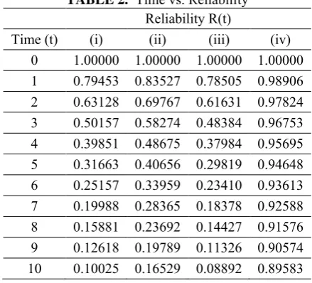
7.2 Reliability Analysis

Letting (i) _λ

0=0.08, λC=0.02, λH=0.05 (ii) λ0=0.02, λC=0.09, λH=0.05 (iii) λ0=0.08, λC=0.08, λH=0.02 (iv) λ0=0.003, λC=0.003, λH=0.002

in (30) and then setting time t=0, 1, 2, 3, 4, 5, 6, 7, 8, 9, 10 unit of time, we get the numerical values of reliability w.r.t. time as presented in Table 2. The same is shown in Figure 3.

TABLE 2. Time vs. Reliability Reliability R(t)

Time (t) (i) (ii) (iii) (iv)

0 1.00000 1.00000 1.00000 1.00000

1 0.79453 0.83527 0.78505 0.98906

2 0.63128 0.69767 0.61631 0.97824

3 0.50157 0.58274 0.48384 0.96753

4 0.39851 0.48675 0.37984 0.95695

5 0.31663 0.40656 0.29819 0.94648

6 0.25157 0.33959 0.23410 0.93613

7 0.19988 0.28365 0.18378 0.92588

8 0.15881 0.23692 0.14427 0.91576

9 0.12618 0.19789 0.11326 0.90574

10 0.10025 0.16529 0.08892 0.89583

0 2 4 6 8 10

0.0 0.2 0.4 0.6 0.8 1.0

7.2(iv)

7.2(iii) 7.2(ii) 7.2(i)

R

el

ia

bi

lit

y

R

(t)

Time (t)

Figure 3. Time vs. Reliability

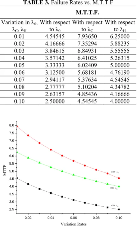
7.3 M.T.T.F. Analysis

Again setting

(i) λC=0.15, λH=0.05 (ii)λ0=0.03, λH=0.06 (iii) λ₀=0.04, λ_C=0.07

in (31) and varying λ0, λC, λH as 0.01, 0.02, 0.03, 0.04, 0.05, 0.06, 0.07, 0.08, 0.09, 0.10 respectively

Figure 4.

TABLE 3.Failure Rates vs. M.T.T.F M.T.T.F.

Variation in λ0, λC, λH

With respect

to λ0

With respect

to λC

With respect

to λH

0.01 4.54545 7.93650 6.25000

0.02 4.16666 7.35294 5.88235

0.03 3.84615 6.84931 5.55555

0.04 3.57142 6.41025 5.26315

0.05 3.33333 6.02409 5.00000

0.06 3.12500 5.68181 4.76190

0.07 2.94117 5.37634 4.54545

0.08 2.77777 5.10204 4.34782

0.09 2.63157 4.85436 4.16666

0.10 2.50000 4.54545 4.00000

0.02 0.04 0.06 0.08 0.10 2.5

3.0 3.5 4.0 4.5 5.0 5.5 6.0 6.5 7.0 7.5 8.0

with  with C

with 

M

T

T

F

Variation Rates

Figure 4. Failure Rates vs. M.T.T.F

8. INTERPRETATION OF THE RESULTS AND CONCLUSION

The graph shown in Figure 2 demonstrates that availability of the system decreases with respect to time when different parameters are given. The availability of the system is high when all the failure rates are very low and also other considered cases of 7.2 when failure in B1or B1is lower than other failures. Observation of Figure 3 reveals that changes in reliability with respect to time corresponding to different situations has almost the same pattern of decrement, but the system seems to be more reliable when failure in unit B1or B1is

lower than other failures. Furthermore it can also be seen from Figure 4 that M.T.T.F. of the system increases with the increase in λ0, λC andλH when other parameters are kept constant.

9. REFERENCES

1. Dhillon, B. S. and Yang, N., “Stochastic analysis of standby systems with common cause failures and human errors”, Microelectron Reliability, Vol. 32, No. 12, (1992), pp. 1699-1712.

2. Gupta, P. P. and Gupta, R. K., “Cost Analysis of an electronic repairable redundant system with critical human error”, Microelectron Reliability, Vol. 26, (1986), pp. 417-421.

3. Jain, M., Kumar, A. and Sharma, G. C., “Maintenance Cost Analysis for Replacement Model with Perfect/Minimal Repair”, International Journal of

Engineering,Vol. 15, No. 2, (2002), pp. 161-168.

4. Jain, M., Maheshwari, R. and Maheshwari S., “Reliability Analysis of Redundant Repairable System with Degraded Failure”, International Journal of

Engineering, Vol. 17, No. 2, (2004), pp. 171-182.

5. Khanduja, R., Tiwari, P. C. and Kumar, D., “Mathematical Modeling and Performance Optimization for the Digesting System of a Paper Plant”,

International Journal of Engineering, Vol. 23, No. 3

& 4, (2010), pp. 215-225.

6. Kontoleon, J. M. and Kontoleon, N., ”Reliability analysis of a system subjected to partial and catastrophic failures”, IEEE Transactions on Reliability, Vol. 23, (1974), pp. 277-278.

7. Nelsen, R. B., “An Introduction to Copulas”, 2nd ed., Springer, New York, (2006).

8. Ram, M. and Singh, S. B., “Availability and Cost Analysis of a parallel redundant complex system with two types of failure under preemptive-resume repair discipline using Gumbel-Hougaard family copula in repair”, International Journal of Reliability, Quality &

Safety Engineering, Vol. 15, No. 4, (2008), pp.

341-365.

9. Ram, M. and Singh, S. B., “Analysis of a Complex System with common cause failure and two types of repair facilities with different distributions in failure”,

International Journal of Reliability and Safety, Vol. 4,

No. 4, (2010), pp. 381-392.

10. Ram, M. and Singh, S. B., “Availability, MTTF and cost analysis of complex system under preemptive-repeat repair discipline using Gumbel-Hougaard family copula”,

, Vol. 27, No. 5, (2010), pp. 576-595. 11. Yang, N. and Dhillon, B. S., “Stochastic analysis of a

general standby system with constant human error and arbitrary system repair rates”, Microelectron

Reliability, Vol. 35, No. 7, (1995), pp. 1037-1045.