TECHNICAL NOTE
MULTI-OBJECTIVE LEAD TIME CONTROL IN MULTISTAGE
ASSEMBLY SYSTEMS
Amir Azaron
Department of Industrial Engineering, University of Bu-Ali Sina, Hamadan, Iran.
S.M.T. Fatemi Ghomi
Department of Industrial Engineering,Amir Kabir University of Technology, Tehran, Iran.
Abstract In this paper we develop a multi-objective model to optimally control the lead time of a multistage assembly system. The multistage assembly system is modeled as an open queueing network, whose service stations represent manufacturing or assembly operations. The arrival processes of the individual parts of the product, which should be assembled to each other in assembly stations, are assumed to be independent Poisson processes with equal rates. In each service station, there is one machine with exponentially distributed processing time, such that the service rate is controllable. The transport times between the service stations are independent random variables with exponential distributions. By applying the longest path analysis in queueing networks, we obtain the distribution function of time spend by a product in the system or the manufacturing lead time. The decision variables of the model are the number of servers in the service stations. The problem is formulated as a multi-objective optimal control problem that involves three conflicting objective functions. The objective functions are the total operating costs of the system per period (to be minimized), the average lead time (min), and the probability that the manufacturing lead time does not exceed a certain threshold (max). The goal programming method is used to solve a discrete-time approximation of the original problem.
Keywords Queueing networks; Optimal control; Production; Multiple objective programming
ﺪﻴﻜﭼ ه ﻲﻟﺪﻣﺎﻣﻪﻟﺎﻘﻣﻦﻳارد
ﻪﻌـﺳﻮﺗياﻪـﻠﺣﺮﻣﺪـﻨﭼژﺎـﺘﻧﻮﻣﻢﺘﺴـﻴﺳﻚـﻳدﺮﺒﺸﻴﭘنﺎﻣزﻪﻨﻴﻬﺑلﺮﺘﻨﻛياﺮﺑﻪﻓﺪﻫﺪﻨﭼ
ﻢﻴﻫدﻲﻣ
. ﺲﻳوﺮـﺳيﺎﻫهﺎﮕﺘﺴﻳانآردﻪﻛدﻮﺷﻲﻣيﺪﻨﺑلﺪﻣزﺎﺑﻒﺻﻪﻜﺒﺷﻚﻳناﻮﻨﻋﻪﺑياﻪﻠﺣﺮﻣﺪﻨﭼژﺎﺘﻧﻮﻣﻢﺘﺴﻴﺳ
ﺖﺳاﺖﺧﺎﺳﺎﻳزﺎﺘﻧﻮﻣتﺎﻴﻠﻤﻋﺮﮕﻧﺎﻴﺑ
.
ﺪﻨﻳاﺮﻓﻪﻛدﻮﺷضﺮﻓ
يﺎﻬﻫﺎﮕﺘﺴـﻳاردﺪـﻳﺎﺑﻪـﻛ،لﻮﺼـﺤﻣيداﺮﻔﻧاتﺎﻌﻄﻗيدورويﺎﻫ
ﻮﭘيﺎﻫﺪﻨﻳاﺮﻓ،ﺪﻧﻮﺷژﺎﺘﻧﻮﻣﺮﮕﻳﺪﻜﻳﻪﺑژﺎﺘﻧﻮﻣ ا
ﺳ ﻮ
ﺪﻨﺘﺴﻫﺮﺑاﺮﺑيﺎﻫخﺮﻧﺎﺑﻞﻘﺘﺴﻣن
.
،ﺲﻳوﺮـﺳهﺎﮕﺘﺴـﻳاﺮـﻫرد
ﻦﻴـﺷﺎﻣﻚـﻳ
دراددﻮﺟو
ﺖـﺳالﺮـﺘﻨﻛﻞـﺑﺎﻗﺲﻳوﺮـﺳخﺮـﻧﻪﻛياﻪﻧﻮﮔﻪﺑ،ﺖﺳاﻲﻳﺎﻤﻧنآشزادﺮﭘﻊﻳزﻮﺗﻪﻛ
.
ـﻣلﺎـﻘﺘﻧايﺎـﻬﻧﺎﻣز
ﻦﻴـﺑﺎ
ﻞﻘﺘﺴﻣﻲﻓدﺎﺼﺗيﺎﻫﺮﻴﻐﺘﻣﺲﻳوﺮﺳيﺎﻬﻫﺎﮕﺘﺴﻳا
ﺪﻨﺘﺴﻫﻲﻳﺎﻤﻧﻊﻳزﻮﺗﺎﺑ
. ردﺮﻴﺴـﻣﻦﻳﺮـﺗﻲﻧﻻﻮـﻃﻞـﻴﻠﺤﺗوﻪﻳﺰﺠﺗدﺮﺑرﺎﻛﺎﺑ
ﻢﻴﻫاﻮـﺧﺖـﺳﺪﺑارﺖﺧﺎﺳدﺮﺒﺸﻴﭘنﺎﻣزﺎﻳﺪﻨﻛﻲﻣفﺮﺻﻢﺘﺴﻴﺳردلﻮﺼﺤﻣﻚﻳﻪﻛﻲﻧﺎﻣزﻊﻳزﻮﺗﻊﺑﺎﺗﺎﻣ،ﻒﺻيﺎﻫﻪﻜﺒﺷ دروآ
. نﺎﮔﺪﻨﻫدﺖﻣﺪﺧداﺪﻌﺗ،لﺪﻣﻢﻴﻤﺼﺗيﺎﻫﺮﻴﻐﺘﻣ
دﻮﺑﺪﻨﻫاﻮﺧﺲﻳوﺮﺳيﺎﻫهﺎﮕﺘﺴﻳارد
. ﻪﻠﺌﺴـﻣﻚـﻳترﻮـﺻﻪﺑﻪﻠﺌﺴﻣ
دﺮﻴﮔﻲﻣﺮﺑردارضرﺎﻌﻣفﺪﻫﻊﺑﺎﺗﻪﺳﻪﻛدﻮﺷﻲﻣيﺪﻨﺑلﻮﻣﺮﻓﻪﻓﺪﻫﺪﻨﺟﻪﻨﻴﻬﺑلﺮﺘﻨﻛ
. يﺎـﻫﻪـﻨﻳﺰﻫﻞـﻛ،فﺪـﻫﻊـﺑاﻮﺗ
دﻮﻳﺮﭘﺮﻫردﻢﺘﺴﻴﺳدﺮﻜﻠﻤﻋ
)
دﻮﺷﻞﻗاﺪﺣﺪﻳﺎﺑﻪﻛ
( ﺮﺒﺸﻴﭘنﺎﻣزﻂﺳﻮﺘﻣ،
)
ﻞﻗاﺪﺣ
( دﺮﺒﺸﻴﭘنﺎﻣزﻪﻜﻨﻳالﺎﻤﺘﺣاو،
زاﺖﺧﺎـﺳ
ﺪﻨﻜﻧزوﺎﺠﺗﻦﻴﻌﻣﺪﺣﻚﻳ
)
ﺮﺜﻛاﺪﺣ
(
دﻮﺑﺪﻨﻫاﻮﺧ،
. ﻲﻧﺎـﻣزﺐـﻳﺮﻘﺗﻚـﻳﺎـﺗدﻮـﺷﻲـﻣﻪﺘﻓﺮﮔرﺎﻛﻪﺑﻲﻧﺎﻣرآيﺰﻳرﻪﻣﺎﻧﺮﺑشور
ﺪﻳﺎﻤﻧﻞﺣارﻲﻠﺻاﻪﻠﺌﺴﻣزاﻪﺘﺴﺴﮔ
1. INTRODUCTION
Over the last decade, manufacturing strategies have focused on speed of response to customer as much as cost and quality for competitive advantage. This means reducing both the length and the variability of the manufacturing lead times. Short lead times are critical to win customer orders for engineer-to-order and make-to-order companies supplying capital goods. These products are often complex assemblies with many stages of manufacture and assembly. Providing competitive delivery lead times and managing to achieve a reliable delivery performance are typically as important as competitive prices.
Each dynamic production system can be modeled as an open queueing network, in which each service station settled in a node of the network represents a manufacturing or assembly operation. It is assumed that one type of product is produced by the system. Each individual part of the product enters the production system according to a Poisson process and goes to the first service station in its routing sequence of manufacturing operations.
In each service station, there is one machine with exponential distribution of processing time. Therefore, the queueing network only contains
M/M/1 queueing systems. The queueing network is
assumed to be in the steady-state and the service rates are controllable.
After completing the manufacturing operations of the individual parts, they are assembled to each other and after passing some other manufacturing and assembly operations, the final product leaves the system in its finished form.
All inter-station buffers are infinite. An implicit hypothesis in the literature is that transit time in buffers is null, i.e., a part which leaves a machine is supposed to be instantaneously available for the next machine. The time needed to cross the inter-section buffers may be much greater than the service time and there is no reason to claim that its effect on the system will be negligible. Therefore, the transport times between the service stations are assumed to be independent random variables with exponential distributions.
The time spent in a service station would be equal to the processing time plus waiting in the queue in front of the service station. Therefore, the time
spend by a finished product in the system would be equal to the length of the longest path of the queueing network whose arc lengths are the transport times between the service stations. We can analytically obtain the distribution function of the manufacturing lead time by computing the distribution function of longest path in the queueing network.
There are many papers about the longest path analysis in stochastic networks, but not queueing networks. Charnes et. al. [3] developed a chance-constrained programming. They assumed exponential activity durations. For polynomial activity durations, Martin [15] provided a systematic way of analyzing the problem through series-parallel reductions. Kulkarni and Adlakha [13] developed an analytical procedure for PERT networks with independent and exponentially distributed activity durations. They modeled such networks as finite-state, absorbing continuous-time Markov chains with upper triangular generator matrices. Then, they proved the time until absorption into this absorbing state is equal to the length of the longest path in the original network provided it starts from the initial state.
Elmaghraby et. al. [5] studied the effect of interactions of different paths on the completion time. Yano [27] considered stochastic lead time in a simple two level assembly system with different processing time distributions including Poisson and negative binomial. Cheng and Gupta [4] and Soroush [24] commented that most analytical studies are limited to small problems. Song et. al.
[23] developed an approximate method to obtain the distribution of product completion time by decomposing the complex product structures of multistage assemblies into two-stage subsystem. The analytical methods above consider the manufacturing and assembly processing times as independent random variables and ignore their dependence on the arrival and service rates of jobs at various stages in the manufacturing process. The time spent in a queue will be longer for congested service stations than for little used stations. Therefore, the time spent waiting in queues in front of service stations should be considered in order to compute the manufacturing lead time.
analysis in dynamic job shops by modelling those as the open queueing networks was studied by Kapadia and Hsi [11], Shanthikumar and Sumita [21], Haskose et. al. [8] and Vandaele et. al. [26]. However, these did not include assembly processes.
Harrison [7] in a primarily theoretical study, introduced a queueing theoretical model of an assembly operation. He established stability conditions for an assembly queue with renewal and mutually independent arrival streams and a single server. Hemachandra and Eedupuganti [9] considered a model of a system with two finite capacity assembly lines and a single join operation and presented an approach for computing the performance measures in the system. Gold [6] considered a model corresponds to an assembly-like queue with two input streams, in which the assembly is instantaneous, and focused on the state probabilities and expectation of minimum and maximum of the two input queues. Ramachandran and Delen [17] analyzed the kitting process (a kit is a set of parts which are all needed to perform the assembly) as of a stochastic assembly system by treating it as an assembly-like queue. Specially, they investigated the dynamics involved in a simple kitting process where two independent input streams feed into an assembly process.
This paper not only considers the manufacturing and assembly processing times as the functions of the arrival and service rates of the various stages of the manufacturing process, but also considers the role of transport times between the service stations, which may be much greater than the processing times, in the manufacturing lead time.
The operator of a plant with service facilities may be regarded as a controller of resources usable in performing services. In fact, we may increase the service rates of the manufacturing and assembly stations by increasing the number of servers. In that case, the average manufacturing lead time will be decreased. However, clearly it causes the total operating costs of the system per period to be increased, accordingly. Consequently, an appropriate trade-off between lead time and cost is required. To achieve the above-mentioned goals, we develop a multi-objective problem to determine the optimum number of servers of the service stations, such that three objectives are sought simultaneously, average lead time (to be
minimized), the probability that the manufacturing lead time does not exceed a certain threshold (max), and also the total operating costs of the assembly system per period (min).
For solving this problem, we do the discretization of time and convert the optimal control problem into an equivalent nonlinear optimization problem. Finally, the goal programming method is used to solve this multi-objective problem.
2. DYNAMIC MULTISTAGE ASSEMBLY SYSTEMS
Each dynamic multistage assembly system can be modeled as an open queueing network, in which each service station settled in a node of the network represents a manufacturing or assembly operation. The following assumptions will be made.
1. Each individual part of the product enters the production system according to a Poisson process with rate
λ
(the demand rate for the final product).2. Only one type of product is produced.
3. Each service station with only one incoming arc indicates a manufacturing station.
4. Each service station with more than one incoming arcs indicates an assembly station. 5. After an individual part arrives in the system, it goes directly to a manufacturing station for its first manufacturing operation. If there are parts for being processed, it queues up.
6. After completion of processing at a manufacturing station, it goes to another manufacturing station to be processed in its routing sequence of manufacturing operations. 7. After completing the manufacturing operations
of each part, it is assembled to some other parts in an assembly station.
8. The product leaves the system in its finished form from the sink node of the queueing network.
9. Each part has characteristics, which are statistically independent of other parts.
10.Each service station consists of one machine. 11.Processing times of manufacturing and
assembly operations are exponentially distributed (including set up times on the service station).
12.The processing time at each service station is independent of preceding processing times. 13.There are no interruptions due to breakdowns,
maintenance, or other such cases. 14.Service discipline is based on FIFO. 15.All inter-station buffers are infinite.
16.The transport times between the service stations are independent random variables with exponential distributions.
17.The queueing network is in the steady-state. 18.The service rates are controllable.
19.Operating cost of each service station per period is an increasing function of its service rate.
20.Total number of service stations settled in the nodes of the queueing network is equal to n. It is clear that the arrival process to the manufacturing stations prior to an assembly station is the Poisson process with the rate of
λ
. Each assembly station has more than one arrival stream, but each assembly operation can begin if and only if the manufacturing operations of all corresponding individual parts, which should be assembled to each other, have been finished. Therefore, it is reasonable to approximate the arrival process to an assembly station, for each set of individual parts available for the assembly operation, as a Poisson process with the rate ofλ
. The arc lengths of the network indicate the transport times between the service stations, which are assumed to be independent random variables with exponential distributions. Consequently, the time spend by a finished product in the system or the manufacturing lead time would be equal to the length of the longest path of the queueing network, in which the length of each node which contains a service station is equal to the time spent in this station.Every two nodes of the queueing network associated with a dynamic multistage assembly system are connected by at most one directed path,
i.e., the network is a tree, and consequently the waiting times in the service stations are independent, see Lemoine [14].
The service rates of the service stations are controllable. The type of service rate control considered here is such that the exponentially distributed processing time, corresponding with the
ith service station, increases from a given average rate
μ
i, when only one server works, to anaverage rate of
k
iμ
i, according to wheneverservers are employed in this service station, in order to minimize the total operating costs of the system per period, minimize the average lead time, and maximize the probability that the manufacturing lead time does not exceed a certain threshold.
i
k
3. LONGEST PATH ANALYSIS IN QUEUEING NETWORKS
In our proposed method, each queueing network is transformed into an equivalent stochastic network with independent and exponentially distributed arc lengths. Then, we determine the distribution function of longest path from the source node to the sink node of this stochastic network by generalizing the method developed by Kulkarni and Adlakha [13].
The main steps of our proposed method are as follows:
Step1. Determine the density function of the time
spent in the service stations. The distribution of waiting time (processing time plus waiting time in queue) in the ith M/M/1 queueing system,
i=1,2,…,n, is
t k i i i i i
e
k
t
w
(
)
=
(
μ
−
λ
)
−( μ−λ) , t>0 (1)where
λ
andk
iμ
i are the arrival rate and the service rate of this queueing system, respectively. Therefore, the distribution of waiting time in theith service station would be exponential with parameter (
k
iμ
i-λ
).Step 2. Transform the queueing network into an
equivalent stochastic network by replacing each node that contains a service station with a stochastic arc whose length is equal to the time spent in the service station.
Let’s explain how to replace node k in the network of queues, which contains a queueing system, with a stochastic arc. Assume that b1,b2,…,bn are the incoming arcs to this node and d1,d2,…,dm are the outgoing arcs from it. Then, we substitute this node by arc (k', k"), whose length is equal to the waiting time in system for the particular queueing system. Furthermore, all arcs bi for i=1,…,n end up with k' while all arcs dj for j=1,…,m start from node k". The indicated process is opposite of the absorption the edge e in the graph G in graph theory (G.e), see Azaron and Modarres [2] for more details. After transforming all such nodes to the stochastic arcs, the queueing network is transformed into an equivalent stochastic network with exponentially distributed arc lengths.
Step 3. Obtain the distribution function of longest
path in the stochastic network obtained in step 2,
using the method of Kulkarni and Adlakha [13].
Let G=(V,A) be a directed stochastic network, in
which V represents the set of nodes and A
represents the set of arcs or the operations of the production system after the transformation. The source and sink nodes are denoted by s and t, respectively. Length of arc is an exponentially distributed random variable with parameter
A a∈
a
γ
. For a∈A, letα
(
a
)
be the starting node of arc a, andβ
(
a
)
be the ending node of arc a. Moreover, I(v) and O(v) arethe sets of arcs ending and starting at node v, respectively, which are defined as follows:{
a A a v}
v
I( )= ∈ :
β
( )= ,(
v
∈
V
)
(2){
a A a v}
v
O( )= ∈ :
α
( )= ,(
v
∈
V
)
(3)Let S denote the set of all admissible 2-partition
cuts of the network, and
S
=
S
∪
{(
φ
,
φ
)}.
It is proven that {X(t),t 0} is a continuous-time Markov process with state space≥
S. The elements of the infinitesimal generator matrix
)}]
'
,
'
(
),
,
{(
[
q
E
F
E
F
Q
=
, (E,F) and)
'
,
'
(
E
F
∈S, are calculated as follows (refer to Kulkarni and Adlakha [13] for details):{
}
{ }
{ }
{ }
{ }
{ }
⎪ ⎪ ⎪ ⎪ ⎪ ⎪ ⎪ ⎩ ⎪⎪ ⎪ ⎪ ⎪ ⎪ ⎪ ⎨ ⎧ = = ∑ γ − β ∪ − = ∪ ⊄ β ∈ γ ∪ = − = ∪ ⊄ β ∈ γ = ) 7 ( 0 ) ' , ' ( ), , ( ) 6 ( ; ' , ' ) 5 ( )) ( ( ) ( ' , )) ( ( , ) 4 ( ; ' , ' , )) ( ( , otherwise F E F E q F F E E if a a O a E E a F a I E a if a a F F a E E a F a I E a if a{X(t),t
≥
0} is a finite-state absorbingcontinuous-time Markov process and since
,
0
)}
,
(
),
,
{(
φ
φ
φ
φ
=
q
it can be concluded that thisstates in S such this Q matrix be an upper triangular one. We assume that the states are
numbered 1,2,…,N=
S
. State 1 is the initial state,namely
(
O
(
s
),
φ
)
, and state N is the absorbing state, namely(
φ
,
φ
)
.Let T represent the length of the longest path in the network, or the manufacturing lead time. It is clear that T=min {t>0: X(t)=N/X(0)=1}. Thus T is the time until {X(t),t
≥
0} gets absorbed in the final state starting from state 1.Chapman-Kolmogorov backward equations is applied to compute F(t)=P{T t} or the distribution function of manufacturing lead time. If we define:
≤
Pi(t)=P{X(t)=N/X(0)=i,}, i=1,2,…,N (8)
Then, F(t)=P1(t).
The system of differential equations for the vector
P(t)=[P1(t),P2(t),…,PN(t)] T
is given by
•
P
(t)=Q.P(t)P(0)=[0,0,…,1]T (9)
where
•
P
(t) represents the derivation of the state vector P(t) and Q is the infinitesimal generator matrix of the stochastic process {X(t),t≥
0}.4. MULTI-OBJECTIVE LEAD TIME CONTROL PROBLEM
In this section we develop a multi-objective model to determine the optimum number of servers in each service station of a multistage assembly system. In fact, we may increase the service rates of the manufacturing and assembly stations by increasing the number of servers. In that case, the average manufacturing lead time will be decreased. However, clearly it causes the total operating costs of the system per period to be increased, accordingly. Consequently, an appropriate trade-off between lead time and cost is required.
To achieve the above-mentioned goals, we develop a multi-objective problem, in which three objectives are sought simultaneously, minimizing average lead time, maximizing the probability that the manufacturing lead time does not exceed a
certain threshold, and also minimizing the total operating costs of the system per period.
The operating cost of the ith service station per period is assumed to be an increasing function
)
(
i ii
k
C
μ
of its service rate,k
iμ
i (μ
i is a givenvalue and is the integer decision variable). Therefore, C or the total operating costs of the system per period can be computed as follows:
i
k
∑
==
n ii i i
k
C
C
1
)
(
μ
(10)The average lead time and the probability that the manufacturing lead time does not exceed a given threshold u are given by
ALT=
∫
∞ − (11)0 (1 P1(t))dt
PR=P1(u) (12)
Taking into account the above assumptions, the infinitesimal generator matrix Q is a function of
the control vector k =
[
k1,k2,...,kn]
T. Therefore, the dynamic model is
•
P
(t)=Q(k).P(t)Pi(0)=0 i=1,2,…,N-1
PN(t)=1 (13)
The relations (14) should be satisfied to exist the response in the steady-state.
i i
k
μ
>λ
, i=1,2,…,n (14)We do not have such constraints in the mathematical programming. Therefore, we use the constraints (15) instead of the above constraints in the final multi-objective problem.
i
k
≥
ε
μ
λ
+
i
, i=1,2,…,n (15)
Assuming as the available number of servers to be allocated to the ith service station, the following set of constraints should also be included in the optimal control problem.
i
U
i
i
U
The appropriate multi-objective lead time control problem would be
Min
∑
=
=
n i i i ik
C
C
1)
(
μ
Min ALT=
∫
∞ −0 (1 P1(t))dt
Max PR=P1(u)
s.t:
•
P
(t)=Q(k).P(t)Pi(0)=0 i=1,2,…,N-1
PN(t)=1
i i i
U
k
≤
≤
+
ε
μ
λ
i=1,2,…,nk Integer (17)
We try to solve problem (17), optimally, using the Maximum Principle, see Sethi and Thompson [20] for the details. For simplicity, we consider only one objective function, for example:
ALT=
∫
∞ − , in the model.0 (1 P1(t))dt
Considering S as the set of allowable controls, which consists of the last set of constraints of problem (17) (k∈S), and n-vector
λ
(
t
)
as the adjoint vector function, the Hamiltonian function would be)
(
1
)
(
)
(
)
(
)
),
(
),
(
(
t
P
t
k
t
Q
k
P
t
P
1t
H
λ
=
λ
T+
−
(18)
Then, we write the adjoint equations and terminal conditions, which are
(19) . , 0 ) ( ], 0 ,..., 0 , 1 [ ) ( ) ( ) ( ∞ → = − + = − • T T k Q t t T T T
λ
λ
λ
If we could compute
λ
(
t
)
from (19), we could minimize the Hamiltonian function subject toin order to get the optimal control , and solve the problem optimally. Unfortunately, the
adjoint equations (19) are dependent on the unknown control vector, k, and therefore they cannot be solved directly.
S
k∈
k
*If we could also minimize the Hamiltonian function (18), subject to , for an optimal control function in closed form as
, then we could substitute
this into the state equations,
S k∈
))
(
),
(
(
* * *t
t
P
f
k
=
λ
•
P
(t)=Q(k).P(t),, and adjoint equations (19) to get a set of differential equations, which is a two-point boundary value problem. Unfortunately, we cannot obtain by differentiating H respect to k, because k is a discrete vector, and consequently cannot be obtained in closed form.
T
P
(
0
)
=
[
0
,
0
,...,
1
]
*
k
*
k
According to the two mentioned points, it is impossible to solve the optimal control problem (17), optimally, even in the case of single objective problem. Relatively few optimal control problems can be solved optimally. Therefore, we try to solve this problem, numerically. To do that, we do the discretization of time and convert the multi-objective discrete optimal control problem into an equivalent multi-objective mixed integer nonlinear programming one. In other words, we transform the differential equations to the equivalent difference equations as well as transform the integral terms into equivalent summation terms. To follow this approach, the time interval is divided into L equal portions with the length of Δt. If Δt
is sufficiently small, it can be assumed that P(t)
varies only in times 0,Δt,…,(L-1) . Considering
P(l
t Δ t
Δ ) as P(l), the continuous-time system
•
P
(t)=Q(k)P(t) is approximated as the followingdiscrete-time system:
P(l+1)=P(l)+Q(k).P(l)Δt l=0,1,…,L-1 (20)
Similarly, ALT is approximated as:
(
∑
=Δ
−
=
L la
P
l
t
ALT
0
1
(
)
1
)
(21)1
)
(
l
≤
P
i , i=1,2,…,N-1, l=1,2,…,L (22)4.1. Goal programming method
Let b1, b2, and b3 represent the goals for the total operating costs, average lead time, and also probability that the manufacturing lead time does not exceed u, respectively. E1, E2, and E3 represent the deviations from the first, second and third goals, respectively. Since E1, E2, and E3 are free variables, then we substitute them with the difference of two nonnegative variables, i.e. Ej=
, j=1,2,3. Let w
− + −
j
j E
E 1, w2,and w3 represent the
importance weights of the deviations from the first, second and third goals, respectively.
Considering
⎢⎣
⎡
⎥⎦
⎤
Δ
t
u
as the integer part of
t
u
Δ
, theappropriate goal programming formulation of the discrete-time approximation of the lead time control problem leads to:
MinZ=
[
( )
( )
( )
]
, 11 3 3 2 2 1
1 + + ≥
+ − − p E w E w E
w p p p p
s.t:
∑
= − +−
=
+
n i i ii
k
E
E
b
C
1 1 1 1)
(
μ
∑
(
)
= − +−
=
+
Δ
−
L lb
E
E
t
l
P
0 2 2 2 1(
)
1
1
(
)
E
3E
3b
3t
u
P
+
−
=
Δ
− +
P(l+1)=P(l)+Q(k)P(l)Δt l=0,1,…,L-1 Pi(0)=0 i=1,2,…,N-1 PN(l)=1 l=0,1,…,L
P
i(
l
)
≤
1
i=1,2,…,N-1, l=1,2,…,Li i i
U
k
≤
≤
+
ε
μ
λ
i=1,2,…,n
k
i:(Integer) i=1,2,…,n(23)
Lemma 1. For , if is an optimal
solution to the optimization problem (23), then is non-dominated.
∞
≤
≤
p
1
k
**
k
If we consider the initial and terminal state
conditions for P(l) implicitly, and substitute each
Pi(0) and PN(l) with zero and one, respectively, nonlinear optimization (23) would have
2L(N-1)+2n+3 constraints, L(N-1)+6 continuous
variables and n integer variables.
For estimating the length of the time interval, we
consider
⎥
⎦
⎤
⎢
⎣
⎡
⎟⎟
⎠
⎞
⎜⎜
⎝
⎛
+
+
=
i i iU
k
μ
ε
λ
5
.
0
for i=1,2,…,n.Then, we solve the system of differential equations (13), analytically, to obtain P1(t). A good estimation for the length of the time interval is
given by
T
ˆ
, where P1(T
ˆ
) should approach one(Tˆ =L.Δt).
A feasible solution, for the discrete-time approximation model, should posses this property that P1(L)≥1−
ε
. If a solution does not have the mentioned property, the value of is increased in order to satisfy this necessary condition.t Δ
5. NUMERICAL EXAMPLE
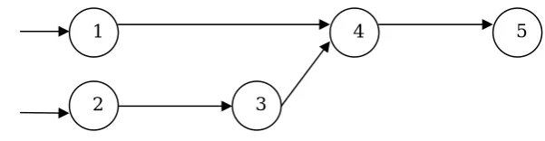
Consider the dynamic assembly system depicted in Figure 1. This system produces chairs. The final chair consists of two separate parts: wooden and leather. In each node, except node 4, there is a manufacturing station with one machine. Node 4 contains an assembly station with one machine. Table 1 shows the characteristics of the service stations (cost unit is in dollar and time unit is in day). We are interested in the optimum number of servers. The other assumptions are as follows: 1. The demand rate for the chair,
λ
, is equal to10 per day.
2. The transport times between the service stations settled in the nodes 1 and 4, and also between those settled in the nodes 3 and 4 are independent exponentially distributed random variables with the parameters
λ
(1,4)=
1
and2
) 4 , 3 (=
λ
. The transport times between the other service stations are zero.1 4
2 3
5
λ
λ
Figure 1. The dynamic assembly system
Table 1. Characteristics of the service stations
Service station Number of servers
C
i(
k
iμ
i)
1 k1 10k1
μ
1+42 k2 4k2
μ
2 +33
k
35
k
3μ
3+
7
4 k4
(
)
2
2 4
4
μ
+
k
5
k
52
k
5μ
5+
5
Now, we transform the queueing network into the equivalent stochastic network with independent and exponentially distributed arc lengths, shown in Figure 2. In this network, the arcs 1, 2 and 4 indicate the waiting times in the M/M/1 queueing systems settled in the nodes 1, 2 and 3 of the queueing network with the parameters (
k
iμ
i-10),for i=1,2,3. The arcs 3 and 5 indicate the transport times between the service stations settled in the nodes 1 and 4 with the parameter 1, and also between the service stations settled in the nodes 3 and 4 of the queueing network with the parameter 2. The arcs 6 and 7 indicate the waiting times in
the M/M/1 queueing systems settled in the nodes 4
and 5 of the queueing network with the parameters (
k
iμ
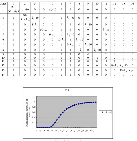
i-10), for i=4,5.The stochastic process {X(t),t 0} related to the longest path analysis of this stochastic network has 14 states. Table 2 shows matrix Q(
≥
μ
),considering
μ
i=
1
for i=1,2,…,n.The length of the time interval is approximated as
. Then, we formulate the appropriate
multi-objective lead time control problem according to (23). The threshold value, u, is assumed to be equal 3. We set the goals for the total operating costs of the system per day, the average lead time and the probability that the manufacturing lead time does not exceed u as b
5 ˆ =
T
1=350 dollars, b2=1.8 days and b3=0.9.Since one day deviation from the average lead time is known to be 100 and 1 times as important as one dollar deviation from the total operating costs of the system per day andone unit deviation from the probability, respectively, then
w1=0.004, w2=w3=0.498. The values of other
parameters are: p=1, L=30, Δt=0.17,
ε
=0.05and
U
i=
15
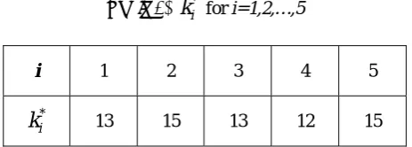
for i=1,2,…,5.Finally, we solve the corresponding problem, using LINGO. Table 3 shows the optimum number of servers in the manufacturing and assembly stations, or for i=1,2,…,5. This solution is a feasible solution, because
F(L)= approaches one
(
*
i
k
) (
1 L
P
986
.
0
)
30
(
L
=
=
F
). Figure 3 shows thedistribution function of lead time F(l) versus
1 4
2 3
5 s
1 3
t
6 7
2 4 5
Figure 2. The stochastic network
Table 2.Matrix Q(k) corresponding to the numerical example
F(l)
0 0.2 0.4 0.6 0.8 1 1.2
0 2 4 6 8 10 12 14 16 18 20 22 24 26 28 30
l
Distribution function o
f
lead time
F(l)
Figure 3.F(l) versus l
State 1 2 3 4 5 6 7 8 9 10 11 12 13 14
1
20-(k1+k2) k2-10 0 0 k1-10 0 0 0 0 0 0 0 0 0
2 0
20-(k1+
k
3) 3k
-10 0 0 0 -10k1 0 0 0 0 0 0 03 0 0 8-k1 2 0 0 0 0 k1-10 0 0 0 0 0
4 0 0 0 10-k1 0 0 0 0 0 0 -10 k1 0 0 0
5 0 0 0 0 9-k2 1 k2-10 0 0 0 0 0 0 0
6 0 0 0 0 0 10-k2 0 k2-10 0 0 0 0 0 0
7 0 0 0 0 0 0 9-
k
3 1k
3-10 0 0 0 0 08 0 0 0 0 0 0 0 10-
k
3 0k
3-10 0 0 0 09 0 0 0 0 0 0 0 0 -3 1 2 0 0 0
10 0 0 0 0 0 0 0 0 0 -2 0 2 0 0
11 0 0 0 0 0 0 0 0 0 0 -1 1 0 0
12 0 0 0 0 0 0 0 0 0 0 0 10-k4 k4-10 0
13 0 0 0 0 0 0 0 0 0 0 0 0 10-
k
5k
5-10Table 3.
k
i* for i=1,2,…,5i 1 2 3 4 5
*
i
k
13 15 13 12 15The total operating costs of the production system per day, the approximated average manufacturing lead time and the approximated probability that the manufacturing lead time does not exceed the given threshold, according to for i=1,2,…,5,
are obtained as follows:
*
i
k
C=450, ALTa=2.2501, PRa=0.8471
6. CONCLUSION
In this paper we developed a new multi-objective model to determine the optimum number of servers to be allocated in the manufacturing and the assembly stations of a dynamic multistage assembly system.
Not only the manufacturing and assembly processing times were considered as the functions of the arrival and service rates of the various stages of the manufacturing process, but also we considered the role of transport times between the service stations in the manufacturing lead time. The corresponding continuous-time problem was so complicated to solve analytically. Therefore, we solved a discrete-time approximation of the original optimal control problem.
To solve the relevant multi-objective problem, we used the goal programming method. This method has some disadvantages; namely, the preferred solution is sensitive to the goal vector and the weighting vector given by the decision maker. However, the goal programming method has fewer variables to work with, so it will be computationally faster. Moreover, according to Lemma 1, for any p greater than or equal 1, the optimal solution of the goal attainment formulation (23) would be a non-dominated or Pareto-optimal solution, refer to Hwang and Masud [10] for the details about multi-objective decision making. Therefore, GP is a good method
to solve our problem, which is complicated to solve even with the presented numerical method. We could also numerically obtain the distribution function of the manufacturing lead time by computing the distribution function of longest path in the queueing network. Seidmann and Smith [19] have developed procedures to assign due-dates for jobs in a job shop environment assuming that the probability distribution of the lead time is known. Therefore, our results complement theirs. Together one may now assign due dates for the final product in a dynamic multistage assembly system.
7. REFERENCES
1. Azaron, A., Fatemi Ghomi, S.M.T., 2003. Optimal Control of Service Rates and Arrivals in Jackson Networks. European Journal of Operational Research 147, 17-31.
2. Azaron, A., Modarres, M., 2005. Distribution Function of the Shortest Path in Networks of Queues. OR Spectrum 27, 123-144.
3. Charnes, A., Cooper, W., Thompson, G., 1964. Critical Path Analysis via Chance Constrained and Stochastic Programming. Operations Research 12, 460-470.
4. Cheng, T.C.E., Gupta, M.C., 1989. Survey of Scheduling Research Involving Due Date Determination decisions. European Journal of Operational Research 38, 156-166.
5. Elmaghraby, S.E., Ferreira, A.A., Tavares, L.V., 2000. Optimal Start Time Under Stochastic Activity Durations. International Journal of Production Economics 64, 153-164. 6. Gold, H., 1998. A Markovian Single Server
with Upstream Job and Downstream Demand Arrival Stream. Queueing Systems 30, 435-455.
7. Harrison, J.M., 1973. Assembly-Like Queues. Journal of Applied Probability 10, 354-367. 8. Haskose, A., Kingsman, B.G., Worthington,
D., 2002. Modelling Flow and Jobbing Shops as a Queueing Network for Workload Control. International Journal of Production Economics 78, 271-285.
in Some Open Assembly Systems. Computers and Operations Research 30, 695-704.
10.Hwang, C., Masud, A., 1979. Multiple Objective Decision Making, Methods and Applications. Springer-Verlag, Berlin.
11.Kapadia, A.S., Hsi, B.P., 1978. Steady State Waiting Time in a Multicenter Job Shop. Naval Research Logistics Quarterly 25, 149-154.
12.Kerbache, L., Smith, J.M., 2000. Multi-Objective Routing within Large Scale Facilities Using Open Finite Queueing Networks. European Journal of Operational Research 121, 105-123.
13.Kulkarni, V., Adlakha, V., 1986. Markov and Markov-Regenerative PERT Networks. Operations Research 34, 769-781.
14.Lemoine, A.J., 1979. On Total Sojourn Time in Networks of Queues. Management Science 25, 1034-1035.
15.Martin, J., 1965. Distribution of the Time Through a Directed Acyclic Network. Operations Research 13, 46-66.
16.Papadopoulos, H.T., Heavey, C., 1996. Queueing Theory in Manufacturing Systems Analysis and Design: A Classification of Models for Production and Transfer Lines. European Journal of Operational Research 92, 1-27.
17.Ramachandran, S., Delen, D., 2005. Performance Analysis of a Kitting Process in Stochastic Assembly Systems. Computers and Operations Research 32, 449-463.
18.Schechner, Z., Yao, D., 1989. Decentralized Control of Service Rates in a Closed Jackson
Network. IEEE Transactions On Automatic Control 34, 236-240.
19.Seidmann, A., Smith, M.L., 1981. Due Date Assignment for Production Systems. Management Science 27, 571-581.
20.Sethi, S., Thompson, G., 1981. Optimal Control Theory. Martinus Nijhoff Publishing, Boston.
21.Shanthikumar, J.G., Sumita, U., 1988. Approximations for the Time Spent in a Dynamic Job Shop with Application to Due-Date Assignment. International Journal of Production Research 26, 1329-1352.
22.Smith, J.M., Daskalaki, S., 1988. Buffer Space Allocation in Automated Assembly Lines. Operations Research 36, 343-358.
23.Song, D.P., Hicks, C., Earl, C.F., 2002. Product Due Date Assignment for Complex Assemblies. International Journal of Production Economics 76, 243-256.
24.Soroush, H.M., 1999. Sequencing and Due-Date Determination in the Stochastic Single Machine Problem with Earliness and Tardiness Costs. European Journal of Operational Research 113, 450-468.
25.Tseng, K., Hsiao, M., 1995. Optimal Control of Arrivals to Token Ring Networks with Exhaustive Service Discipline. Operations Research 43, 89-101.
26.Vandaele, N., Boeck, L.D., Callewier, D., 2002. An Open Queueing Network for Lead Time Analysis. IIE Transactions 34, 1-9. 27.Yano, C.A., 1987. Stochastic Lead-Time in