APPROXIMATE DYNAMIC ANALYSIS OF STRUCTURES
FOR EARTHQUAKE LOADING USING FWT
A. Heidari*
Faculty of Engineering, University of Shahrekord Shahrekord, Iran
E. Salajegheh
Department of Civil Engineering, University of Kerman Kerman, Iran
*Corresponding Author
(Received: March 16, 2006 - Accepted: March 18, 2007)
Abstract Approximate dynamic analysis of structures is achieved by fast wavelet transform (FWT). The loads are considered as time history earthquake loads. To reduce the computational work, FWT is used by which the number of points in the earthquake record are reduced. For this purpose, the theory of wavelets together with filter banks are used. The low and high pass filters are used for the decomposition of earthquake records in the high and low frequency of the records. The low frequency content is the most important part; therefore this part of the record is used for dynamic analysis. A number of structures are analysed and the results are compared with exact dynamic analysis and the Fast Fourier method (FFT).
Keywords Approximate Dynamic Analysis, Signal Processing, Filter Banks, Fast Wavelet Transforms
ﻩﺪﻴﻜﭼ
ﻩﺯﺎﺳﻲﺒﻳﺮﻘﺗﻞﻴﻠﺤﺗﻪﻟﺎﻘﻣﻦﻳﺍﺭﺩ
ﺑﺭﺩﺎﻫ
ﺖﺳﺍ ﺮﻈﻧﺩﺭﻮﻣﻲﻜﺟﻮﻣﻊﻳﺮﺳﻞﻳﺪﺒﺗﺯﺍﻩﺩﺎﻔﺘﺳﺍﺎﺑﻪﻟﺰﻟﺯﺮﺑﺍﺮ
.
ﻲﺷﺎﻧﻱﻭﺮﻴﻧ،ﻩﺯﺎﺳﺮﺑﻲﻟﺎﻤﻋﺍﺭﺎﺑ
ﺯﺍ
ﻪﺘﻓﺮﮔﺮﻈﻧﺭﺩﻪﻟﺰﻟﺯ
ﻲﻣﻡﺎﺠﻧﺍﻲﻧﺎﻣﺯﺔﭽﺨﻳﺭﺎﺗﻞﻴﻠﺤﺗﻩﺯﺎﺳﻱﺍﺮﺑﻭﻩﺪﺷ
ﺩﻮﺷ
.
ﻲﻣﻩﺩﺎﻔﺘﺳﺍﻲﻜﺟﻮﻣﻊﻳﺮﺳﻞﻳﺪﺒﺗﺯﺍﻪﻟﺰﻟﺯﻁﺎﻘﻧﺩﺍﺪﻌﺗﺶﻫﺎﻛﻭﻱﺮﺗﻮﻴﭙﻣﺎﻛﺕﺎﺒﺳﺎﺤﻣﺶﻫﺎﻛﻱﺍﺮﺑ
ﺩﻮﺷ
.
ﻦﻳﺍﻱﺍﺮﺑ
ﻲﻣﻩﺩﺎﻔﺘﺳﺍﺎﻫﺮﺘﻠﻴﻓﻭﺎﻬﻜﺟﻮﻣﻱﺭﻮﺌﺗﺯﺍﺭﻮﻈﻨﻣ
ﺩﻮﺷ
.
ﻦﻴﻳﺎﭘﻭﻻﺎﺑﻱﺎﻫﺮﺘﻠﻴﻓﺯﺍ
ﺏﺎﺘﺷﻪﻳﺰﺠﺗﻱﺍﺮﺑﺭﺬﮔ
ﻪﻟﺰﻟﺯﺖﺷﺎﮕﻧ
ﻲﻣﻩﺩﺎﻔﺘﺳﺍﻲﻨﺤﻨﻣﻭﺩﻪﺑ
ﺩﻮﺷ
.
ﻲﻨﺤﻨﻣﻦﻳﺍﺯﺍﻲﻜﻳ
ﺲﻧﺎﻛﺮﻓﻞﻣﺎﺷﺎﻫ
ﺲﻧﺎﻛﺮﻓﻞﻣﺎﺷﻱﺮﮕﻳﺩﻭﻪﻟﺰﻟﺯﻦﻴﺋﺎﭘﻱﺎﻫ
ﻱﺎﻫ
ﺖﺳﺍﻥﺁﻱﻻﺎﺑ
.
ﺲﻧﺎﻛﺮﻓ
ﺍﺭﻪﻟﺰﻟﺯﺓﺪﻤﻋﺖﻤﺴﻗﻦﻴﺋﺎﭘﻱﺎﻫ
ﻞﻴﻜﺸﺗ
ﻩﺯﺎﺳﻲﻜﻴﻣﺎﻨﻳﺩﻞﻴﻠﺤﺗﻱﺍﺮﺑﺎﻬﻧﺁﺯﺍﻦﻳﺍﺮﺑﺎﻨﺑ،ﻩﺩﺍﺩ
ﻲﻣﻩﺩﺎﻔﺘﺳﺍ
ﺩﻮﺷ
.
ﻭﻖﻴﻗﺩ ﻞﻴﻠﺤﺗ ﺯﺍﻩﺩﺎﻔﺘﺳﺍﺎﺑﻥﺁ ﺞﻳﺎﺘﻧﻭﻩﺪﺷ ﻞﻴﻠﺤﺗﺵﻭﺭ ﻦﻳﺍ ﺎﺑﻪﻟﺰﻟﺯ ﺮﺑﺍﺮﺑ ﺭﺩﻩﺯﺎﺳﻱﺩﺍﺪﻌﺗ
ﺵﻭﺭ FFT
ﻲﻣﻪﺴﻳﺎﻘﻣ
ﺩﻮﺷ
.
1. INTRODUCTION
Time history dynamic analysis of the structures for earthquake loads is, in general, time consuming and the computational cost of the process is high [1]. For large-scale problems, the computational time for time history analysis is excessive in particular. This makes the structure analysis process very inefficient, especially when a time history analysis is considered.
By Fourier Transform (FT), a signal can be expressed as the sum of a series ( possibly infinite)
of sines and cosines. This sum is also referred to as a Fourier expansion [1]. The disadvantage of FT, however is that it has only frequency resolution and no time resolution [2]. To overcome this problem, in the past decades several solutions have been developed which are more or less able to represent a signal in the time and frequency domain simoultaniously [3]. Another disadvantage of the FT is that it cannot separate the low and high frequencies [4].
of the FT [5]. In the WT the use of a fully scalable window solves the signal-cutting problem. The window is shifted along the signal and for every position the spectrum is calculated. Then this process is repeated many times with a slightly shorter (or longer) window for every new cycle. In the end the result will be a collection of time-frequency representations of the signal, all with different resolutions [2]. In the WT we normally speak about time-scale representations, scale being in a way the opposite of frequency [6].
There are three kinds of wavelet transforms, continuous wavelet transforms (CWT) [7], discrete wavelet transforms (DWT) [8] and fast wavelet transforms (FWT) [9]. In references [10,11] the DWT is used for dynamic analysis. Then the DWT is used for optimisating structures for the earthquake induced loading [12-14].
In the present study, the FWT is used for dynamic analysis. The FWT is used to transfer the ground acceleration record of the specified earthquake into a signal with a very small number of points. Thus the time history dynamic analysis is carried out at fewer points. The earthquake record is broken into multi level records. The original record passes through two complementary filters and emerges as two signals. For many earthquake records, the low frequency content is the effective part, because most of the energy of the record is in the low frequency part. On the other hand, for a record, the shape and the effects of the entire low frequency component are similar to those of the main record. For an earthquake record if the high frequency components are removed, the record is different, but the pattern of the record can still be distinguished. However, if the low frequency components are removed, the record is different, and the main record cannot be distinguished. The numerical results of the dynamic analysis show that this approximation is a powerful technique and the required computational work can be reduced greatly. The error involved in the FWT is small.
2. BASIC FEATURES OF SIGNAL PROCESSING
There are two kinds of signal processing, one is continuous signal processing (CSP) and the other
is discrete signal processing (DSP). According to the Shanon sampling theory, each CSP can be converted into DSP [15] therefore we focus on DSP. In the signal processing theory, each point of a signal is called a sample or point. Discrete time signals are represented mathematically as a sequence of numbers.
One of the important system classes consists of those that are linear and time-invariant (LTI). The combination of these two properties leads to convenient representations for such systems. This class of systems is defined by the principle of superposition. From the principle of superposition and the property of time-invariance, it can be written [14]:
∑ +∞
−∞
= −
=
k
) k t ( h ) k ( s )
t (
y (1)
As a consequence of Equation 1, a LTI system is completely characterized by its impulse response h(t) in the sense that, given h(t), it is possible to use Equation 1 to compute the output y(t) due to any input s(k). Equation 1 is commonly called the convolution sum [15]. This equation will be used for filtering the earthquake record in the subsequent sections.
3. CONTINUOUS WAVELET TRANSFORMS
FT is an example of basis functions used in function approximation. If a function is piecewise smooth, with isolated discontinuities, the FT is poor because of discontinuities. The WT are well suited to approximate piece-wise smooth signals. There is an important difference between FT and WT. The Fourier basis (sines and cosines) are localized in frequency but not in time, the WT is local in both frequency and time.
Like the FT (time-frequency representation) the complete WT process creates three-dimensional representation with description of time, scale, and amplitude of the WT coefficients. The WT decomposes a time series into time-scale space and enables one to determine both dominant modes of variability and how those modes vary in time. The CWT is performed by projecting a signal s(t) into a family of zero-mean functions deduced from an elementary function ψ(t) by translations and dilations as follows [7]:
∫ +∞ ∞ − ∗ ψ
= s(t) a,b(t)dt )
b , a (
CWT (2)
where the symbol * denotes the complex conjugate, and ψa,b(t) is a wavelet and defined as:
) a b t ( 5 . 0 a ) t ( b , a − ψ − =
ψ (3)
The wavelets ψa,b(t) are generated from a single basic wavelet ψ(t) that is called the mother wavelet by scaling and translation, a is the scaling factor, b represents the translation and the factor
5 . 0
a− is for energy normalization across different scales. Equation 2 shows how signal s is decomposed into a set of basic functions ψa,b(t). For large a, the basic function becomes stretched, while for small a, the basic function becomes a contracted wavelet. The most important properties of wavelets are the admissibility and the regularity of conditions and these are the properties that gave wavelets their name.
The variable a is the scale factor and controls the scale of the wavelet, so that taking |a| > 1 dilates the wavelet ψ, and taking |a| < 1 compresses ψ. The variable b is the time translation factor and controls the position of the wavelet. The wavelet
transform is characterized by the following properties:
1. It is a linear transformation, 2. It is covariant under translations:
) u t ( s ) t (
s → − CWT(a,b)→CWT(a,b−u)
3. It is covariant under dilations:
) kt ( s ) t (
s → CWT(a,b)→k−0.5CWT(ka,kb)
The basic difference between WT and FT is that when the scale factor a is changed, the duration and the bandwidth of the wavelet are both changed, but its shape remains the same. The CWT uses short windows at high frequencies and long windows at low frequencies, in contrast to FT, which uses a single analysis window. This partially overcomes the time resolution limitation of FT. CWT can also be assumed as a filter bank analysis composed of band-pass filters with a constant relative bandwidth. If CWT(a,b) is the WT of a signal s(t), then s(t) can be restored using the formula:
∫ ∞−+∞∫ ∞−+∞ ψ − −
− ψ
= )a 2dadb
a b t ( ) b , a ( CWT 1 . C ) t ( s (4)
providing that the FT of wavelet ψ(t), denoted by )
v (
ψ satisfies the following admissibility conditions:
∫ ∞−+∞ − <∞
=
ψ ψ(v) 2v 1dv
C (5)
which shows that ψ(v), has to oscillate and decay.
4. DISCRETE WAVELET TRANSFORMS
WT has no analytical solutions and they can be calculated only numerically. To overcome these problems DWT has been introduced. This is achieved by modifying the wavelet representation in Equation 3 by:
) j 0 a j 0 a 0 kb t ( j 5 . 0 o a ) t ( k ,j − ψ − =
ψ (6)
then the DWT of Equation 2 is:
∫ +∞ ∞ − ∗ ψ = s(t) ,jk(t)dt )
k ,j (
DWT (7)
where j and k are integers and a0 > 1 is a fixed dilation step. The translation factor b0 depends on the dilation step. The effect of discretizing the wavelet is that the time-scale space is now sampled at discrete intervals. If the DWT is used to transform a signal, the result will be a series of wavelet coefficients.
5. FAST WAVELET TRANSFORMS
In FWT, a scaling function corresponding to the mother wavelet is used. In the FWT two signals are computed. Detail signals Dj and approximate signal Aj are obtained as follows:
K ..., , 2 , 1 k J ..., , 2 , 1 j
t k)
j 2 t ( j h ) t ( s ) t ( j D = = ∑ ∗ − = (8) K ..., , 2 , 1 k J ..., , 2 , 1 j n ) k j 2 t ( j g ) t ( s ) t ( j A = = ∑ ∗ − = (9)
where h stands for high pass and g stands for low pass filters, the wavelets and scaling functions must be deduced from one stage to the next. Consider two filter impulse responses g(t) and h(t), the wavelets and the scaling functions are obtained iteratively as: ∑ − = + k ) k 2 t ( 1 g ) k ( j g ) t ( 1 j
g (10a)
∑ −
= +
khj(k)g1(t 2k) )
t ( 1 j
h (10b)
It can be seen that for all the decomposed records the total time is the same as the original record but the number of points is reduced.
The FWT corresponds to the analysis of the filter bank, whereas the inverse fast wavelet transform (IFWT) corresponds to the synthesis one. The filters presented in the IFWT are precisely h~(t) and g~(t). The IFWT achieves multi resolution decomposition of s(t) on J stage labelled by j = 1, …, J, given by;
∑ = ∑ − + ∑= ∑ − = J 1 j k ) k j 2 t ( j g~ ) t ( j A J 1 j ) k j 2 t ( j h ~ ) t ( j D k ) t ( s (11)
where h~j(t−2jk) is called the synthesis wavelets and g~j(t−2jk) is called the synthesis scaling functions [9]. The h~ and g~ are used for high and low pass filters, respectively.
6. FILTERS USED TO CALCULATE FWT AND IFWT
All the filters used in the FWT and IFWT are intimately related to the sequence Ǘ φ(t). Clearly if φ(t) is compactly supported, the sequence φ(t) is finite and can be viewed as a filter. The filter
) t (
φ , which is called the scaling filter, is a low pass filter, and has a length of 2N, a sum of 1, a norm of (1/ 2), LTI, and has only a finite number of nonzero samples [9]. From filter φ(t), we define four filters, of length 2N and norm 1. The four filters are computed using the following scheme.
) t ( g~ ) t ( g )) t ( h ~ ( QMF ) t ( g~ ) t ( h ~ ) t ( h ) t ( ) t ( ) t ( h ~ − = → = ↓ − = → φ φ =
and h~ and g~ are used in the IFWT to reconstruction. The QMF is a quadrature mirror filter, and defined as [9]:
N 2 ,... 2 , 1 k ) k 1 N 2 ( h ~ 1 k ) 1 ( ) k (
g~ = − + + − = (12)
7. THE FWT TO APPROXIMATE EARTHQUAKE RECORDS
In the FWT, at each level of transformation, the signal is processed through a low pass and a high pass filter. The high pass filtered signal is known as the detail wavelet coefficients. The result of the low pass transform is then decimated by a factor of two and used as input signal at the next level of resolution. After the decimation, the same two filters are applied to the data. The process of decomposition is repeated until the resulting error is in the specified limit. In the present work an error of less than 10 percent for maximum difference is allowed.
For a record s(t) with Np points, the complete FWT consists of log2Np stages at most. The decomposition starts from the original record s(t), and produces two sets of signals; detail signals D1, and approximate signals A1. In each stage, the record is divided into two parts, the first part contains the high frequencies and the other contains the low frequencies. The main steps in the process of time history dynamic analysis of structures for a specified earthquake record employing the FWT are as follows:
• The functions ψ and φ are defined. In this study, the Haar wavelet and the associate scaling function are selected [8].
• The number of stages for decomposition of the record is chosen. In this paper four stages (j = 1, …, 4) are used. The numerical results indicate that the error in the 4th stage of decomposition is not acceptable.
• The FWT of the earthquake record in the first stage is computed. Convolving X obtains these vectors with the low pass filter for A1 (by Equation 9), and with the high pass filter for D1 (by Equation 8), respectively.
• Then from signal A1, the two signals A2 and D2 are evaluated and the process is continued until AJ and DJ are evaluated. For the earthquake record, the approximation record (Aj) with low frequency components is the effective part [15].
• The approximate version of the earthquake record in all stages (namely Aj) is used for dynamic analysis.
• The dynamic responses of the structure for Aj record are calculated by Newmark beta method [1].
• The actual responses of the structure are calculated by IFWT using Equation 11. The algorithm is invertible and the signal can be reconstructed iteratively from the detail coefficients together with the last level coefficients of the low pass filter.
In step (f) the dynamic responses of the structures is calculated by the Newmark beta method that is considered a generalization of the linear acceleration method [1]. This method is employed for a step-by-step numerical integration of motion of a multi degree freedom system. The dynamic equilibrium equation of the structures is as:
) t ( j A u MI ) t ( Ky ) t ( y C ) t ( y
M&& + & + = (13)
where M, C and K are mass, damping and stiffness matrixes of the structure, respectively. The vectors
y&&, y& and y are acceleration, velocity and
displacements of the degrees of freedom, respectively. Iu is the unit matrix and Aj is the acceleration record. In this paper, Aj is calculated by Equation 9. The mass and stiffness matrixes are computed by the characteristics of the members of the structure and the damping matrix is computed by the help of the mass and stiffness matrixes. In the Newmark beta method, the structure is analysed and the values of y&&, y&and y are calculated at all the time steps of the record. Then the member forces and stresses in the structure under consideration can be easily calculated employing y&&, y&and y.
Figure 1. Shear building of 7 stories.
TABLE 1. Results of Maximum Displacement of Example. Maximum dynamic displacement (cm) Floor No.
EDA FFT A1 A2 A3 A4
1 1.952 1.963 1.975 2.035 2.082 2.153 2 3.758 3.796 3.859 3.928 3.972 4.058 3 5.459 5.509 5.554 5.611 5.631 5.676 4 7.027 7.016 7.008 7.045 7.017 6.981 5 8.353 8.272 8.270 8.174 8.094 7.966 6 9.340 9.297 9.168 8.945 8.830 8.623 7 9.876 9.764 9.626 9.334 9.203 8.952 is the same for all the filtered records, but the time
intervals are not the same. On the other hand, the direct integration method by the Newmark beta method is carried out at less number of points with different time steps.
8. NUMERICAL EXAMPLES
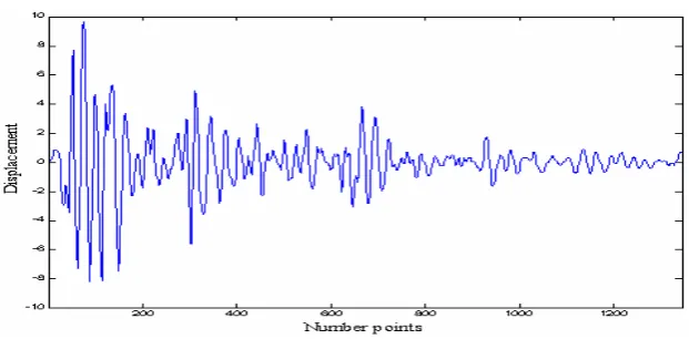
Two examples are analysed for the El Centro Earthquake record (S-E 1940). The Haar wavelet is used for the FWT. The number of points of the El Centro is 2688, and the time interval is 0.02 seconds. The exact response of structure is calculated by the Newmark beta method. A personal computer Pentium 4 is used and the computing time is calculated by clock time. The analysis is carried out by the following methods:
1. Exact dynamic analysis (EDA) 2. Dynamic analysis using the FFT
3. Dynamics analysis with the FWT by signals A1, A2, A3, A4.
8.1. Problem 1. Plane shear building
The plane shear building model of 7 stories shown in Figure 1, is analysed, with the assumption that the floor masses only move horizontally. It is assumed that the mass of each rigid floor of the model includes the effect of the masses of all the structural elements adjacent to the floor of the prototype building. The mass of each floor is 90 tons. Thematerial properties are given as Young’s modulus, E = 2 × 10⁶ kg/cm2, weight density, ρ = 0.0078 kg/cm3 anddamping ratio for all modes as 0.2. The moments of inertia for all columns are 2 × 104 cm4. Results of the analysis for maximum displacement of each floor for all cases for the El Centro record are given in Table 1. The displacement history of the top storey, for the El Centro record for exact dynamic analysis, and dynamic analysis by A1, A2, A3 and A4 records are shown in Figures 2 to 6.
Figure 2. Displacement history of level 7 by EDA (cm).
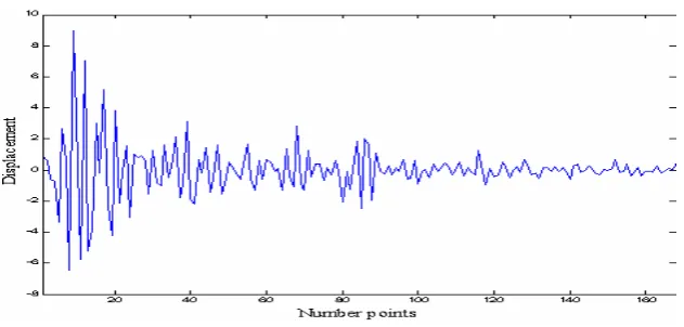
Figure 3. Displacement history of level 7 by A1 (cm).
Figure 4. Displacement history of level 7 by A2 (cm). are similar. The time of computation in EDA is
greater than FFT, FFT is greater than A1, A1 is greater than A2, A2 is greater than A3, and A3 is greater than A4. For the El Centro record the time of analysis for EDA, FFT, A1, A2, A3 and A4 are
Figure 5. Displacement history of level 7 by A3 (cm).
Figure 6. Displacement history of level 7 by A4 (cm).
8.2. Problem 2
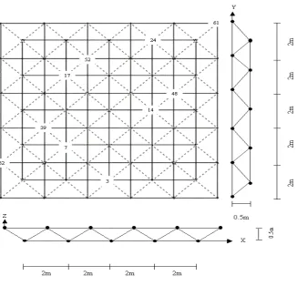
A double layer grid of the type shown in Figure 7 is chosen with dimensions of 10×10 m for top layer and 8×8 m for the bottom layer. The height of the structure is 0.5 m and is simply supported at the corners of the bottom layer. The material properties are given as Young’s modulus, E = 2.1×10⁶ kg/cm2, weight density, ρ = 0.008 kg/cm3 and a damping ratio for all modes as 0.1. The cross sections of all members are 15 cm2. The mass density of the material is assumed to be 0.001 kg-s2/cm4 and the mass of 10 kg-s2/cm is lumped at each free node. Results of the analysis of maximum displacements of joints 3, 7, 14, 17, 24, 32, 39, 48,52 and 61 for directions X, Y and Z, for the El Centro record are given in Tables 2 to 4, respectively.
9. CONCLUSIONS
From the numerical results presented in this paper and a number of other structures [16], the following points can be concluded:
Figure 7. Double layer grid.
• The overall time required for dynamic analysis is reduced substantially using FWT. • In each successive decomposition, the time of
analysis is reduced by a factor of nearly 2 but the error is increased by a factor of 2.
• The best choice for approximation record is the second and third stages of decomposition (A2 and A3), because, the error of computation is acceptable.
• By FWT we can separate the low and the high frequency of the record. The low frequency of record is important, because it contains most of the energy of the record and the shape of the low frequency is similar to the shape of the main record. Therefore we can analyse the structure against this part. The results are almost similar to those of the original earthquake record. The error is negligible, in particular in the first stages of decomposition.
10. REFERENCES
1. Paz, M., “Structural Dynamics: Theory and Computation”, McGraw Hill, New York, (1997).
2. Polikar, R., “The wavelet tutorial. http://users. rowan.edu/~polikar/WAVELETS/WTtutorial. html”, (2001).
3. Thuillard, M., “Wavelets in Soft Computing”, World
Scientific Publishing Co. Pte. Ltd., New York, (2001). 4. Strang, G. and Nguyen, T., “Wavelets and Filter
Banks”, Wellesley-Cambridge Press, New York, (1996).
5. Stanislaw, R. M., “Wavelet analysis for Processing of
Ocean Surface Wave Records”, Ocean Engineering,
Vol. 28, (2001), 957-987.
6. Farge, M., “Wavelet Transforms and their Application
to Turbulence”, Annual Reviews Fluid Mechanics,
Vol. 24, (1992), 395-457.
7. Morlet, J., “Sampling theory and Wave Propagation”,
In: Proceedings of the 5lst Annu. Meet. Soc. Explor. Geophys, Los Angeles, (1981).
8. Daubechies, I., “Ten Lectures on Wavelets. CBMS-NSF
TABLE 2. Maximum Dsplacement of Eample 2 (X Drection). Maximum dynamic displacement * 10-2 Joints No.
EDA FFT A1 A2 A3 A4
3 106 106 105 110 109 83 7 107 106 105 109 104 88 14 104 105 105 107 101 83 17 106 107 106 105 103 88 24 94 93 92 93 94 85 32 115 116 119 117 112 99 39 81 80 79 77 81 75 48 72 73 71 73 72 67 52 87 87 85 89 84 70 61 79 78 77 72 69 73
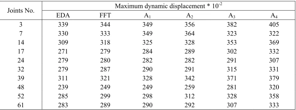
TABLE 3. Maximum Displacement of Example 2 (Y Direction). Maximum dynamic displacement * 10-2 Joints No.
EDA FFT A1 A2 A3 A4
3 102 103 105 112 116 125 7 94 95 97 98 89 92 14 91 93 93 94 98 110 17 58 56 55 51 57 71 24 56 55 54 52 54 65 32 62 63 59 56 52 76 39 56 56 55 50 47 54 48 57 58 54 54 48 46 52 64 61 60 58 53 59 61 53 52 51 49 45 44
TABLE 4. Maximum Displacement of Example 2 (Z Direction). Maximum dynamic displacement * 10-2 Joints No.
EDA FFT A1 A2 A3 A4
(1992).
9. Mallat, S., “A Theory for Multiresolution Signal
Decomposition: the Wavelet Representation”, IEEE
Transactions on Pattern Analysis and Machine Intelligence, Vol. 11, (1989), 674-693.
10. Salajegheh, E. and Heidari, A., “Dynamic Analysis of Structures Against Earthquake by Combined Wavelet Transform and Fast Fourier Transform”, Asian Journal of Civil Engineering, Vol. 3, (2002), 75-87.
11. Salajegheh, E. and Heidari, A., “Time History Dynamic Analysis of Structures Using Filter Banks and Wavelet
Transforms”, Computers and Structures, Vol. 83,
(2005), 53-68.
12. Salajegheh E. and Heidari A., “Optimum Design of Structures Against Earthquake by Wavelet Transforms
and Filter Banks”, International Journal of
Earthquake Engineering and structural Dynamics,
Vol. 34, (2004), 67-82.
13. Salajegheh, E. and Heidari, A., “Optimum Design of Structures Against Earthquake by Adaptive Genetic
Algorithm Using Wavelet Networks”, Structural and
Multidisciplinary Optimization, Vol. 28, (2004),
277-285.
14. Salajegheh, E., Heidari, A. and Saryazdi, S., “Optimum Design of Structures Against Earthquake by Discrete
Wavelet Transform”, International Journal for
Numerical Methods in Engineering, Vol. 62, (2005),
2178-2192.
15. Oppenheim, A. V., Schafer, R. W. and Buck, J. R., “Discrete-Time Signal Processing”, Prentice Hall, New Jersey, USA, (1999).