Please cite this article as: S. Ajeel Fenjan, H. Bonakdari, A. Gholami, A. A. Akhtari, Flow Variables Prediction Using Experimental, Computational Fluid Dynamic and Artificial Neural Network Models in a Sharp Bend, International Journal of Engineering (IJE), TRANSACTIONS A: Basics..Vol. 29, No. 1, (January 2016) 14-22
International Journal of Engineering
J o u r n a l H o m e p a g e : w w w . i j e . i rFlow Variables Prediction Using Experimental, Computational Fluid Dynamic and
Artificial Neural Network Models in a Sharp Bend
S. Ajeel Fenjan, H. Bonakdari*, A. Gholami, A. A. Akhtari Department of Civil Engineering, Razi University, Kermanshah, Iran
P A P E R I N F O
Paper history:
Received 13 March 2015
Received in revised form 24 January 2016 Accepted in 28 January 2016
Keywords:
Computational Fluid Dynamics Model Artificial Neural Network Model 90° Sharp Bend
Flow Velocity Flow Pressure
A B S T R A C T
Bend existence causes changes in the flow pattern, velocity and the water surface profile. The ability to simulate three-dimensional flow pattern is an important and significant issues in curved channel. In the present study, using three-dimensional model of computational fluid dynamics (CFD) and artificial neural network (ANN) model of multi-Layer perceptron (MLP), two velocities and pressure variables on the channel bed with 90º sharp bend is predicted and compared. Also extensive experimental work has been conducted to measure the flow variables in this bend. Experimental results are used to train and test the neural network model accordingly. Comparison of the numerical with experimental results show that CFD model with average Root Mean Square Error (RMSE), 0.02 and 0.13 and ANN model with R2 (determination coefficient) value, 0.984 and 0.99 to predict velocity and pressure respectively, has reasonable accuracy. Also, velocity pattern and flow pressure with both numerical (CFD and ANN) models at any point of the field channel is predictable. Comparison of the CFD and ANN models show that the ANN model with the average value of Mean Absolute Error (MAE), 0.048 to CFD model with the average MAE, 0.06 in prediction of velocity and pressure has more accuracy. The present neural network with less time and cost in designing and implementation of curved channels than other expensive and time consuming experimental and computational models can be used.
doi: 10.5829/idosi.ije.2016.29.01a.03
1. INTRODUCTION1
In the path of rivers and artificial channels can be seen that there are several curves which caused considerable difficulties in understanding the flow pattern in this path. Therefore, the characteristics of the flow in this region are great importance of hydraulic researchers. The numerical and experimental studies have been done a lot in this area. Blanckaert and Graf [1] carried out wide experimental investigations on a 120° sharp bend, and paid the pattern of turbulent flow in the bend. The results showed that the lack of shear stresses coordination in the cross-section led to the formation of the secondary rotating cell near the outer bend of 60° cross section. Lu et al. [2] did numerical study in a 180° curved channel. The researchers found that in the
*Corresponding Author’s Email: [email protected] (H. Bonakdari)
shear stress distribution, streamlines, velocity contours and secondary flow formation was studied as well. The result is considered as the maximum velocity position and displacement. They stated that the maximum velocity in sharp bends to the end sections of the bend remains in the vicinity of the inner wall. There are many other numerical studies about channels [7-11].
In recent decades, artificial intelligence methods in addition to reduce the computation time, are able to predict the flow parameters in all conditions, especially in places where experimental data are not available. Therefore, in recent years the useing of these methods has a special place among water engineers [12-21]. A MLP model is a type of artificial neural network used for predicting variables.Sahu et al. [22], used artificial neural networks to study and predict the velocity profiles in open channel meanders. The correlation coefficient between results showed the efficiency and accuracy of the neural network model to predict the velocity. Bonakdari et al. [23] predicted the velocity field values in a mild bend using ANN and the Genetic Algorithm. They used three-dimensional numerical modeling to verify the results where no experimental results were available. Their results indicated that there is an acceptable level of consistency between the results of the numerical and ANN models. Baghalian et al. [24] took a sediment tool into account and studied the flow in a 90° mild bend. According to their results, the numerical and ANN models were more consistent with the experimental values compared with the analytical solution. Gholami et al. [25] predicted two velocity and water surface variables in 90º sharp bend using both CFD and MLP models. They decared that the ANN model perform more accurate than CFD model.
In this study, the two variables velocity and channel bed pressure is investigated at 90° sharp bend by using two different numerical models (CFD and ANN) which is rarely addressed in previous studies. First, a computational fluid dynamics model is used to investigate the three-dimensional flow pattern in sharp bends. In the end, two artificial neural network models is trained to based on available experimental data to predict the flow velocity and pressure. The performance of these models to predict the velocity and channel bed pressure are assessed by using three statistical parameters: R2, RMSE, and MAE.
2. GOVERNING EQUATIONS
Governing equations are the equations of continuity and momentum equations in the incompressible turbulent flow with viscosity and constant density as an average of the time can be expressed as follows:
0 )
(
U div
t
(1)
( ) 1
i
i i i
j x i j
j i j j
u u P u
u g u u
t x x x x
(2)
) (j i
u
= The velocity component in the direction i (j), P= total pressure, ρ = Density of the fluid, ν= molecular viscosity,i
x
g = gravitational acceleration in the direction
j
x and uiuj= the Reynolds stresses that apply turbulence effect on the fluid.
3.NUMERICAL AND EXPERIMENTAL MODELS
The desired solution field is consistent with the available experimental model, the channel details are a 90° curved channel with two straight channels in the upstream and downstream. The length of upstream 3.6m and downstream channel 2m is considered and the dimensions of the rectangular channel is 30cm×40.3cm (height and width of the channel); the central angle of bend is 90° and central radius is 60.45 cm (Rc= 60.45cm), according to the
channel width (b = 40.3cm) bend is sharp (Rc/b= 1.5<3).
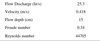
Bed and walls of the channel are fix and made of Plexiglas, and manning coefficient is n=0.008, so the cross section is hydraulically smooth. To measure the longitudinal velocity, the PROPLER one-dimensional velocity meter was used. The flow height was measured with a micrometer. The micrometre measured the depth with 0.1 mm precision and the velocity with 2 cm/s precision [6, 26]. Flow hydraulic characteristics are shown in Table 1. Considering the Froude number= 0.34 and Reynolds number=44705, flow regime is subcritical and turbulent. Figure 1 is shown a view of the experimental flume.
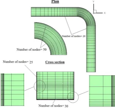
To construct the numerical model, as shown in Figure 2 the geometry of the flow field created in the software Gambit then to adjust the grid of flow field near the channel bed, walls, inside the bend and also at the interface of the two phases finer gridding and in other areas larger gridding is considered. In general, network with 73,346 nodes is generated. In the present numerical model, for closure equations, k(RNG) turbulence model is used.
TABLE 1. Hydraulic characteristic of the tests
Flow Discharge (lit/s) 25.3
Velocity (m/s) 0.418
Flow depth (cm) 15
Froude number 0.34
Figure 1. The geometry of the experimental model
Figure 2. Gridding of 90° bend in plan and cross-section
Boundary condition for the flow entrance is Velocity
Inlet that for the water and air phase is considered
separately. Free surface boundary condition Pressure
Inlet in the case of two-phase flow, the outlet boundary
condition Pressure Outlet in the open channel state and
free surface level, and boundary condition of the bed and
the walls Wall have been considered.
4. ARTIFICIAL NEURAL NETWORK (ANN) MODEL
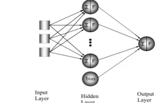
Implementation of the amazing features of the brain in an artificial system is always tempting and desirable. Generally, an artificial neural network composed of interconnected nodes called neurons, that in three basics layers input, hidden, and output are arranged. Neurons in each layer are connected to the neurons of the next layer by weights. In this study, the multi-layer perceptron neural network (MLP-NN) is used. The flexible structure of MLP in simulation of nonlinear problems with their high efficiency causes the widespread use of this model in practical conditions [13, 27]. The structure of a multi-layer perceptron consists of
one input layer and one or more hidden layers and one output layer is shown in Figure 3.
The MATLAB R2011b software is utilized to prepare a proper neural network model. The input layer introduces the input variables to the model with neurons and transmits them to the hidden layer. The hidden layer gatters the input layer neurons by using a weighted summation and so transmits them to a non-linear future by activation functions. MLP models often use sigmoid activation functions [28, 29]. Any function that has a proportional relation between the input and output variables is a sigmoid function. In the present study, the hyperbolic tangent activation function is used for the hidden layer (Equation (1)) [30]:
1 e 1
2 tanh(x) 2x
(3)
experimental data. The model should converge for each number of epochs. In the present study, given that the MLP models converged at 100 epochs, the number of epochs considered was 100.
• At the ANN model for velocity prediction: In this study, a total of 320 experimental data were used to train the network, of which 225 and 95 data have been used to train and test the network, respectively. • At the ANN model for bed pressure prediction: 104
experimental data (75 data for training and 29 data for testing the network) is used. Cross sections, points located on the each cross section, and the distance from the channel bed (z) are shown in Figure 4. For the velocity network, this points in three distance from the bed of the channel (z = 3, 6, and 9 cm) and for the pressure network points at the bed of the channel network (Z = 0) are used.
5. RESULTS AND DISCUSSION
5. 1. Statistical Indices In the present study, to better compare experimental data and the results of numerical models, some error criterion is used. "Root Mean Square Error" is briefly called RMSE indicates the difference between the estimated and measured data is obtained from Equation (4), the other way "determination coefficient" or R2 according to Equation (5) and "Mean Absolute Error" is called MAE for short, is obtained from Equation (6):
N t O RMSE
N
i i i
1
2
(4)
N
i
i i N
i i i
O O
t O R
1
2 1
2
2
1 (5)
N
i i
i t
O N MAE
1
1
(6)
In these equations, N is the number of measurement points, ti experimental measured data and Oipredicted by
the model andOthe mean of the model values. The lower
RMSE and MAE value and the greater value of R2, indicating the high accuracy of the model was estimated and predicted more consistent with experimental data. The RMSE and MAE values show the difference between experimental and numerical values by the same scale and unit and as the values are closer to zero, the model accuracy will be high.
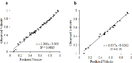
5. 2. Model Performance Evaluation Figures 5 and 6 show the correlation analysis between the velocity values and the bed pressure values predicted by the ANN
model and the experimental data in train and test states, respectively. The RMSE and R2 is shown above each figure. At the Figures 5 and 6, it can be seen that all data on both sides of the line fitted with a 45º angle have been largely symmetrical. Also, shown in Figure 5, in train state, R2equal to 0.9834 and the network test state, the R2
value is equal to 0.984. At the bed pressure prediction network, the R2values at the train and test states are 0.9883 and 0.99, respectively. Due to the proximity of the
R2 value in the train and test states, can be concluded that both obtained ANN models are not been over train. In this figure, linear fitted line equation with y=C1x+C2 is used.
The value of C1 and C2 is closer to 1 and the value of C2
is closer to 0, the proposed model is more accurate. The given values of C1 in Figure 5 at the train and test state
are 1.0121 and 1.006, respectively. Also, the amount of C2 in this relationship are 0.0018 and 0.0113 that can
contribute to the accuracy of ANN model to predict the velocity in train and test states, respectively. In Figure 6, the values of C1, at the train and test states are 1.0121 and
1.006, respectively, and the value of C2 in this
relationship are 0.0018 and 0.0113, respectively, which indicate the accuracy of the ANN model to predict the pressure on the bed of the channel in the train and test states. Given these values, we find that both ANN models are well-trained and their performance in predicting the velocity and the channel bed pressure are satisfactory.
Figure 3. Multi- layer perceptron network general diagram
5. 3. Models Comparison In Figure 7, the longitudinal velocity distribution simulated by CFD and ANN models have been compared with experimental data in different cross sections in the Z = 3cm level (near the channel bed). In Table 2, the RMSE and MAE
values have been collected for the velocity transverse profiles between the results obtained from the CFD and ANN models with experimental data in different cross sections. According to figures, the CFD results with experimental results coincide with the RMSE average value of 0.0205 and MAE, 0.018. The RMSE value of 0.008 and MAE of 0.006 between ANN model results with experimental data shows high accuracy of ANN model in predicting velocity. In Figure 8, the transverse pressure profiles predicted by CFD and ANN models are compared with experimental data on the channel bed in 8 cross section. In Table 2, the amount of error (RMSE and MAE) is given between the predicted results of pressure distribution in different cross sections (Figure 8). Be careful of these values, can be seen that the CFD model with RMSE, 0.13 and MAE, 0.11 cm in accordance with experimental results is acceptable.
The CFD model with the RMSE average value of 0.12 and MAE, 0.11 acts well in prediction of pressure variable. With the arrival to the bend, due to the centrifugal force creation, transverse slope of the water surface decreases at the inner wall of the channel and increases at the outer wall.
Figure 5. Comparison of velocity values predicted by the CFD model and experimental model in: a- Train and b- Test states
Figure 6. Comparison of pressure values predicted by the ANN model and experimental model in: a- Train and b- Test states
Figure 7. Comparison of transverse profiles of longitudinal velocity at: a- CFD model with experimental data and b- ANN model with experimental data
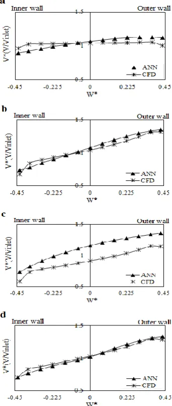
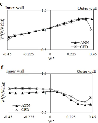
The pressure value is equal to height of water surface multiple in specific gravity (p= γ×h), where p, the pressure, h, water surface height and γ specific gravity of the water is equal 9810 (N / m2). Therefore, the pressure changes are like water surface changes pattern in channel bed. So, in the inner cross sections, the maximum pressure occures in the outer wall and the minimum pressure occures in the inner wall of the channel. This process creates transverse pressure gradient within the cross section of the channel. As in the channel bed, pressure gradient overcomes to the centrifugal force and at the water surface, the centrifugal force to the pressure gradient, and so the rotational cell is created in channel cross section. This rotational flow is moved to the inner wall at the channel bed and to the outer wall at the water surface. This rotational cell called secondary flow phenomena that are typical subjects of the curved channels. As previously mentioned, a neural network has been trained and ensured their performance. In this section, we will study the velocity distribution by ANN model in the points which no experimental data are available and then to compare these values with the values obtained by the CFD simulations. In this study, the experimental data obtained only in 8 sections but neural network can study the velocity and water depths values in other sections. In Figures 9, the depth averaged velocity distribution are predicted in the different cross sections by the ANN and CFD model and compared by each other.
TABLE 2. Comparing velocity and pressure distribution in the CFD and ANN model with the experimental model at Z = 3cm from the channel bed at different cross sections
Velocity Prediction Pressure Prediction
CFD model ANN model CFD model ANN model
Cross Section RMSE MAE RMSE MAE RMSE MAE RMSE MAE
40 cm before 0.026 0.023 0.008 0.006 0.0048 0.0047 0.0047 0.0045
0° 0.029 0.024 0.0075 0.006 0.12 0.09 0.10 0.09
22.5° 0.03 0.027 0.006 0.005 0.096 0.087 0.11 0.09
45° 0.027 0.025 0.005 0.004 0.12 0.096 0.12 0.094
67.5° 0.022 0.019 0.0055 0.003 0.22 0.2 0.24 0.20
90° 0.01 0.01 0.0123 0.008 0.15 0.105 0.14 0.095
40 cm after 0.009 0.008 0.008 0.0055 0.13 0.12 0.127 0.1
80 cm after 0.0115 0.009 0.0102 0.008 0.165 0.164 0.176 0.17
Averaged Values 0.0205 0.018 0.008 0.006 0.13 0.10 0.127 0.09
Figure 9. Comparing depth averaged velocity distribution in the CFD and ANN model at: (a) 30 cm before the bend, (b) 20°, (c) 30°, (d) 50°, (e) 70°, and (f) 30 cm after the bend cross sections
TABLE 3. Comparing pressure distribution in the CFD and ANN model at channel bed at different cross sections
Cross Section RMSE (cm) MAE (cm)
30 cm before the bend 0.068 0.06
20° 0.048 0.043
30° 0.207 0.2
40° 0.05 0.043
50° 0.031 0.026
60° 0.034 0.028
70° 0.08 0.04
30 cm after the bend 0.096 0.09
Averaged Values 0.08 0.066
Another point to note is that in the present sharp bend, the position of the maximum velocity is often in the inner portion of bend because of longitudinal flow power and its dominance on the secondary flow in these bends.
6. CONCLUSION
In the present study, experimental model, finite volumes numerical model and neural network model are used to predict the velocity and channel bed pressure at a 90° sharp bend. For this purpose, at first the numerical computational fluid dynamics model is used to simulate the bend’s flow pattern. The two multi-layer perceptron
neural network (MLP-NN) models have been trained to predict the velocity and pressure of channel bed. Acceptable compliance of the both CFD and ANN numerical models results with experimental model represents the high accuracy of numerical models in prediction of two velocity and flow pressure variables in 90º sharp bend. Both models predict the velocity and pressure pattern on the channel bed as well. In sharp bends, the maximum velocity is happened in the inner wall and moves to outer wall of channel in the sections located after the bend which is predicted well by two CFD and ANN models. However, in comparison of two models, it can be said that the ANN model with less error value than the CFD model perform more accurate. Both models can also predict the flow variables values in other parts and cross sections of channel which there is no experimental data, accordingly. The ANN model with time-consuming and less expensive than the CFD model is able to predict the flow velocity and pressure at each point of the channel.
7. REFERENCES
1. Blanckaert, K. and Graf, W.H., "Mean flow and turbulence in open-channel bend", Journal of Hydraulic Engineering, Vol. 127, No. 10, (2001), 835-847.
2. Lu, W., Zhang, W., Cui, C. and Leung, A., "A numerical analysis of free-surface flow in curved open channel with velocity–pressure-free-surface correction", Computational Mechanics, Vol. 33, No. 3, (2004), 215-224.
3. Bodnár, T. and Příhoda, J., "Numerical simulation of turbulent free-surface flow in curved channel", Flow, turbulence and combustion, Vol. 76, No. 4, (2006), 429-442.
4. Zhang, M.-l. and Shen, Y.-m., "Three-dimensional simulation of meandering river based on 3-D rng κ-ɛ turbulence model",
Journal of Hydrodynamics, Ser. B, Vol. 20, No. 4, (2008), 448-455.
5. Naji, A.M., Ghodsian, M., Vaghefi, M. and Panahpur, N., “Experimental and numerical simulation of flow in a 90° bend”,
Flow Measurement and Instrumentation, Vol. 21, No. 3, (2010), 292-298
6. Gholami, A., Akbar Akhtari, A., Minatour, Y., Bonakdari, H. and Javadi, A.A., "Experimental and numerical study on velocity fields and water surface profile in a strongly-curved 90° open channel bend", Engineering Applications of Computational Fluid Mechanics, Vol. 8, No. 3, (2014), 447-461.
7. Bonakdari, H. and Zinatizadeh, A.A., "Influence of position and type of doppler flow meters on flow-rate measurement in sewers using computational fluid dynamic", Flow Measurement and Instrumentation, Vol. 22, No. 3, (2011), 225-234.
8. Mignot, E., Bonakdari, H., Knothe, P., Lipeme Kouyi, G., Bessette, A., Rivire, N. and Bertrand-Krajewski, J., "Experiments and 3d simulations of flow structures in junctions and their influence on location of flowmeters", Water Science and Technology, Vol. 66, No. 6, (2012), 1325.
10. Bonakdari, H., Ebtehaj, I. and Azimi, H., "Numerical analysis of sediment transport in sewer pipe", International Journal of Engineering-Transactions B: Applications, Vol. 28, No. 11, (2015), 1564-1570.
11. Sharifipour, M., Bonakdari, H. and Zaji, A., "Impact of the confluence angle on flow field and flowmeter accuracy in open channel junctions", International Journal of Engineering-Transactions B: Applications, Vol. 28, No. 8, (2015), 1145-1153.
12. Hadian, M.R., Zarrati, A. and Eftekhari, M., "Development of an implicit numerical model for calculation of sub-and super-critical flows", International Journal of Engineering Transactions B: Applications,, Vol. 18, No. 1, (2005), 85-95. 13. Bilhan, O., Emiroglu, M.E. and Kisi, O., "Application of two
different neural network techniques to lateral outflow over rectangular side weirs located on a straight channel", Advances in Engineering Software, Vol. 41, No. 6, (2010), 831-837. 14. Emiroglu, M.E., Bilhan, O. and Kisi, O., "Neural networks for
estimation of discharge capacity of triangular labyrinth side-weir located on a straight channel", Expert Systems with Applications, Vol. 38, No. 1, (2011), 867-874.
15. Goel, A. and Pal, M., "Stage-discharge modeling using support vector machines", International Journal of Engineering Transactions A: Basics, Vol. 25, No. 1, (2012), 1-9.
16. Mirzaei, E., Minatour, Y., Bonakdari, H. and Javadi, A., "Application of interval-valued fuzzy analytic hierarchy process approach in selection cargo terminals, a case study",
International Journal of Engineering-Transactions C: Aspects, Vol. 28, No. 3, (2014), 387-296.
17. Bahramifara, A., Shirkhanib, R. and Mohammadic, M., "An anfis-based approach for predicting the manning roughness coefficient in alluvial channels at the bank-full stage",
International Journal of Engineering-Transactions B: Applications,, Vol. 26, No. 2, (2013), 177-186.
18. Haji, M.S., Mirbagheri, S., Javid, A., Khezri, M. and Najafpour, G., "A wavelet support vector machine combination model for daily suspended sediment forecasting", International Journal of Engineering-Transactions C: Aspects, Vol. 27, No. 6, (2013), 855-864.
19. Zaji, A.H. and Bonakdari, H., "Application of artificial neural network and genetic programming models for estimating the longitudinal velocity field in open channel junctions", Flow Measurement and Instrumentation, Vol. 41, No., (2015), 81-89.
20. Gholami, A., Bonakdari, H., Zaji, A.H., Akhtari, A.A. and Khodashenas, S.R., "Predicting the velocity field in a 90° open channel bend using a gene expression programming model",
Flow Measurement and Instrumentation, Vol. 46, (2015), 189-192.
21. Yuhong, Z. and Wenxin, H., "Application of artificial neural network to predict the friction factor of open channel flow",
Communications in Nonlinear Science and Numerical Simulation, Vol. 14, No. 5, (2009), 2373-2378.
22. Sahu, M., Jana, S., Agarwal, S., Khatua, K. and Mohapatra, S., "Point form velocity prediction in meandering open channel using artificial neural network", in Proceedings of International Conference on Environmental Science and Technology (2011). 23. Bonakdari, H., Baghalian, S., Nazari, F. and Fazli, M.,
"Numerical analysis and prediction of the velocity field in curved open channel using artificial neural network and genetic algorithm", Engineering Applications of Computational Fluid Mechanics, Vol. 5, No. 3, (2011), 384-396.
24. Baghalian, S., Bonakdari, H., Nazari, F. and Fazli, M., "Closed-form solution for flow field in curved channels in comparison with experimental and numerical analyses and artificial neural network", Engineering Applications of Computational Fluid Mechanics, Vol. 6, No. 4, (2012), 514-526.
25. Gholami, A., Bonakdari, H., Zaji, A.H. and Akhtari, A.A., "Simulation of open channel bend characteristics using computational fluid dynamics and artificial neural networks",
Engineering Applications of Computational Fluid Mechanics, Vol. 9, No. 1, (2015), 355-369.
26. Akhtari, A., Abrishami, J. and Sharifi, M., "Experimental investigations water surface characteristics in strongly-curved open channels", Journal of Applied Sciences, Vol. 9, No. 20, (2009), 3699-3706.
27. Kim, S., Shiri, J. and Kisi, O., "Pan evaporation modeling using neural computing approach for different climatic zones", Water Resources Management, Vol. 26, No. 11, (2012), 3231-3249. 28. Zadeh, M.R., Amin, S., Khalili, D. and Singh, V.P., "Daily
outflow prediction by multi layer perceptron with logistic sigmoid and tangent sigmoid activation functions", Water Resources Management, Vol. 24, No. 11, (2010), 2673-2688. 29. Ebtehaj, I. and Bonakdari, H., "Evaluation of sediment transport
in sewer using artificial neural network", Engineering Applications of Computational Fluid Mechanics, Vol. 7, No. 3, (2013), 382-392.
30. Dawson, C.W. and Wilby, R., "An artificial neural network approach to rainfall-runoff modelling", Hydrological Sciences Journal, Vol. 43, No. 1, (1998), 47-66.
31. Kisi, O. and Kerem Cigizoglu, H., "Comparison of different ann techniques in river flow prediction", Civil Engineering and Environmental Systems, Vol. 24, No. 3, (2007), 211-231. 32. Levenberg, K., "A method for the solution of certain non–linear
Flow Variables Prediction Using Experimental, Computational Fluid Dynamic and
Artificial Neural Network Models in a Sharp Bend
S. Ajeel Fenjan, H. Bonakdari, A. Gholami, A. A. Akhtari Department of Civil Engineering, Razi University, Kermanshah, Iran
P A P E R I N F O
Paper history:
Received 13 March 2015
Received in revised form 24 January 2016 Accepted in 28 January 2016
Keywords:
Computational Fluid Dynamics Model Artificial Neural Network Model 90° Sharp Bend
Flow Velocity Flow Pressure
هديكچ
یم بآ حطس و تعرس لیفورپ ،نایرج یوگلا رد رییغت بجوم سوق دوجو .ددرگ
یدعب هس نایرج یوگلا یزاس هیبش ییاناوت
ایس کیمانید یدعب هس لدم زا هدافتسا اب ،رضاح قیقحت رد .دشاب یم هدیمخ یاه لاناک رد هجوت لباق و مهم تاعوضوم زا تلا
لدم و یتابساحم دنت سوق لاناک فک رب دراو راشف و تعرس رییغتم ود ،نورتپسرپ ی هیلا دنچ یبصع هکبش
09 شیپ هجرد
یم هسیاقم و ینیب هدش ماجنا سوق نیا رد نایرج یاهرییغتم یریگ هزادنا رد یا هدرتسگ یهاگشیامزآ تاقیقحت نینچمه .دوش
آ یارب دوجوم یهاگشیامزآ جیاتن زا .تسا یاهلدم زا لصاح جیاتن ی هسیاقم .دوش یم هدافتسا یبصع هکبش لدم تست و شزوم
ربارب اطخ تاعبرم روذجم طسوتم رادقم اب یتابساحم تلاایس کیمانید لدم هک دهد یم ناشن یهاگشیامزآ جیاتن اب یددع
90 / 9 و 31 / 9 صیخشت بیرض رادقم اب یبصع هکبش لدم و 089
/ 9 و 00 / 9 شیپ یارب هب ینیب نایرج راشف و تعرس بیترت
.دنراد یلوبق لباق تقد تعرس یوگلا نینچمه
راشف و یددع لدم ود ره کمک هب نایرج یتابساحم تلاایس کیمانید(
هکبش و
یبصع )یعونصمم شیپ لباق لح نادیم زا هطقن ره رد یم ینیب
.دشاب هکبش لدم هک دهد یم ناشن مه اب لدم ود نیا ی هسیاقم
قلطم یاطخ طسوتم رادقم اب یبصع 998
/ 9 قلطم یاطخ طسوتم اب تلاایس کیمانید لدم هب تبسن 90
/ 9 شیپ رد تعرس ینیب
اناک یارجا و یحارط رد رتمک ی هنیزه و تقو فرص اب رضاح یبصع هکبش لدم زا ناوت یم .دراد یرتشیب تقد راشف و یاه ل
.درک هدافتسا یتابساحم و یهاگشیامزآ ریگ تقو و نارگ یاهلدم رگید یاجب هدیمخ