R E S E A R C H
Open Access
Adaptive lifting scheme with sparse criteria for
image coding
Mounir Kaaniche
1*, Béatrice Pesquet-Popescu
1, Amel Benazza-Benyahia
2and Jean-Christophe Pesquet
3Abstract
Lifting schemes (LS) were found to be efficient tools for image coding purposes. Since LS-based decompositions depend on the choice of the prediction/update operators, many research efforts have been devoted to the design of adaptive structures. The most commonly used approaches optimize the prediction filters by minimizing the variance of the detail coefficients. In this article, we investigate techniques for optimizing sparsity criteria by focusing on the use of anℓ1criterion instead of anℓ2one. Since the output of a prediction filter may be used as an input for the other prediction filters, we then propose to optimize such a filter by minimizing a weightedℓ1 criterion related to the global rate-distortion performance. More specifically, it will be shown that the optimization of the diagonal prediction filter depends on the optimization of the other prediction filters and vice-versa. Related to this fact, we propose to jointly optimize the prediction filters by using an algorithm that alternates between the optimization of the filters and the computation of the weights. Experimental results show the benefits which can be drawn from the proposed optimization of the lifting operators.
1 Introduction
The discrete wavelet transform has been recognized to be an efficient tool in many image processing fields, including denoising [1] and compression [2]. Such a success of wavelets is due to their intrinsic features: multiresolution representation, good energy compaction, and decorrelation properties [3,4]. In this respect, the second generation of wavelets provides very efficient transforms, based on the concept of lifting scheme (LS) developed by Sweldens [5]. It was shown that interesting properties are offered by such structures. In particular, LS guarantee a lossy-to-lossless reconstruction required in some specific applications such as remote sensing imaging for which any distortion in the decoded image may lead to an erroneous interpretation of the image [6]. Besides, they are suitable tools for scalable recon-struction, which is a key issue for telebrowsing applica-tions [7,8].
Generally, LS are developed for the 1D case and then they are extended in a separable way to the 2D case by cascading vertical and horizontal 1D filtering operators. It is worth noting that a separable LS may not appear always very efficient to cope with the two-dimensional
characteristics of edges which are neither horizontal nor vertical [9]. To this respect, several research studies have been devoted to the design of non separable lifting schemes (NSLS) in order to better capture the actual two-dimensional contents of the image. Indeed, instead of using samples from the same rows (resp. columns) while processing the image along the lines (resp. col-umns), 2D NSLS provide smarter choices in the selec-tion of the samples by using horizontal, vertical and oblique directions at the prediction step [9]. For exam-ple, quincunx lifting schemes were found to be suitable for coding satellite images acquired on a quincunx sam-pling grid [10,11]. In [12], a 2D wavelet decomposition comprising an adaptive update lifting step and three consecutive fixed prediction lifting steps was proposed. Another structure, which is composed of three predic-tion lifting steps followed by an update lifting step, has also been considered in the nonadaptive case [13,14].
In parallel with these studies, other efforts have been devoted to the design of adaptive lifting schemes. Indeed, in a coding framework, the compactness of a LS-based multiresolution representation depends on the choice of its prediction and update operators. To the best of our knowledge, most existing studies have mainly focused on the optimization of the prediction stage. In general, the goal of these studies is to * Correspondence: [email protected]
1Télécom ParisTech, 37-39 rue Dareau 75014 Paris, France Full list of author information is available at the end of the article
introduce spatial adaptivity by varying the direction of the prediction step [15-17], the length of the prediction filters [18,19] and the coefficient values of the corre-sponding filters [9,11,15,20,21]. For instance, Gerek and Çetin [16] proposed a 2D edge-adaptive lifting scheme by considering three direction angles of prediction (0°, 45°, and 135°) and by selecting the orientation which leads to the smallest gradient. Recently, Ding et al. [17] have built an adaptive directional lifting structure with perfect reconstruction: the prediction is performed in local windows in the direction of high pixel correlation. A good directional resolution is achieved by employing fractional pixel precision level. A similar approach was also adopted in [22]. In [18], three separable prediction filters with different numbers of vanishing moments are employed, and then the best prediction is chosen according to the local features. In [19], a set of linear predictors of different lengths are defined based on a nonlinear function related to an edge detector. Another alternative strategy to achieve adaptivity aims at design-ing liftdesign-ing filters by defindesign-ing a given criterion. In this context, the prediction filters are often optimized by minimizing the detail signal variance through mean square criteria [15,20]. In [9], the prediction filter coeffi-cients are optimized with a least mean squares (LMS) type algorithm based on the prediction error. In addi-tion to these adaptaaddi-tion techniques, the minimizaaddi-tion of the detail signal entropy has also been investigated in [11,21]. In [11], the approach is limited to a quincunx structure and the optimization is performed in an empirical manner using the Nelder-Mead simplex algo-rithm due to the fact that the entropy is an implicit function of the prediction filter. However, such heuristic algorithms present the drawback that their convergence may be achieved at a local minimum of entropy. In [21], a generalized prediction step, viewed as a mapping func-tion, is optimized by minimizing the detail signal energy given the pixel value probability conditioned to its neighbor pixel values. The authors show that the result-ing mappresult-ing function also minimizes the output entropy. By assuming that the signal probability density function (pdf) is known, the benefit of this method has firstly been demonstrated for lossless image coding in [21]. Then, an extension of this study to sparse image representation and lossy coding contexts has been pre-sented in [23]. Consequently, an estimation of the pdf must be available at the coder and the decoder side. Note that the main drawback of this method as well as those based on directional wavelet transforms [15,17,22,24,25] is that they require to transmit losslessly a side information to the decoder which may affect the whole compression performance especially at low bitrates. Furthermore, such adaptive methods lead to an
increase of the computational load required for the selection of the best direction of prediction.
It is worth pointing out that, in practical implementa-tions of compression systems, the sparsityof a signal, where a portion of the signal samples are set to zero, has a great impact on the ultimate rate-distortion per-formance. For example, embedded wavelet-based image coders can spend the major part of their bit budget to encode the significance map needed to locate non-zero coefficients within the wavelet domain. To this end, sparsity-promoting techniques have already been investi-gated in the literature. Indeed, geometric wavelet trans-forms such as curvelets [26] and contourlets [27] have been proposed to provide sparse representations of the images. One difficulty of such transforms is their redun-dancy: they usually produce a number of coefficients that is larger than the number of pixels in the original image. This can be a main obstacle for achieving effi-cient coding schemes. To control this redundancy, a mixed contourlet and wavelet transform was proposed in [28] where a contourlet transform was used at fine scales and the wavelet transform was employed at coarse scales. Later, bandlet transforms that aim at developing sparse geometric representations of the images have been introduced and studied in the context of image coding and image denoising [29]. Unlike contourlets and curvelets which are fixed transforms, bandelet trans-forms require an edge detection stage, followed by an adaptive decomposition. Furthermore, the directional selectivity of the 2D complex dual-tree discrete wavelet transforms [30] has been exploited in the context of image [31] and video coding [32]. Since such a trans-form is redundant, Fowler et al. applied a noise-shaping process [33] to increase the sparsity of the wavelet coefficients.
With the ultimate goal of promoting sparsity in a transform domain, we investigate in this article techni-ques for optimizing sparsity criteria, which can be used for the design of all the filters defined in a non separ-able lifting structure. We should note that sparsest wavelet coefficients could be obtained by minimizing an
ℓ0 criterion. However, such a problem is inherently non-convex and NP-hard [34]. Thus, unlike previous studies where prediction has been separately optimized by mini-mizing anℓ2criterion (i.e., the detail signal variance), we focus on the minimization of an ℓ1criterion. Since the output of a prediction filter may be used as an input for other prediction filters, we then propose to optimize such a filter by minimizing a weighted ℓ1 criterion related to the global prediction error. We also propose
to jointly optimize the prediction filters by using an
criterion is often considered in the signal processing lit-erature such as in the compressed sensing field [35], it is worth pointing out that, to the best of our knowledge, the use of such a criterion for lifting operator design has not been previously investigated.
The rest of this article is organized as follows. In Sec-tion 2, we recall our recent study for the design of all the operators involved in a 2D non separable lifting structure [36,37]. In Section 3, the motivation for using anℓ1 criterion in the design of optimal lifting structures is firstly discussed. Then, the iterative algorithm for minimizing this criterion is described. In Section 4, we present a weightedℓ1 criterion which aims at minimiz-ing the global prediction error. In Section 5, we propose to jointly optimize the prediction filters by using an algorithm that alternates between optimizing all the fil-ters and redefining the weights. Finally, in Section 6, experimental results are given and then some conclu-sions are drawn in Section 7.
2 2D lifting structure and optimization methods
2.1 Principle of the considered 2D NSLS structure
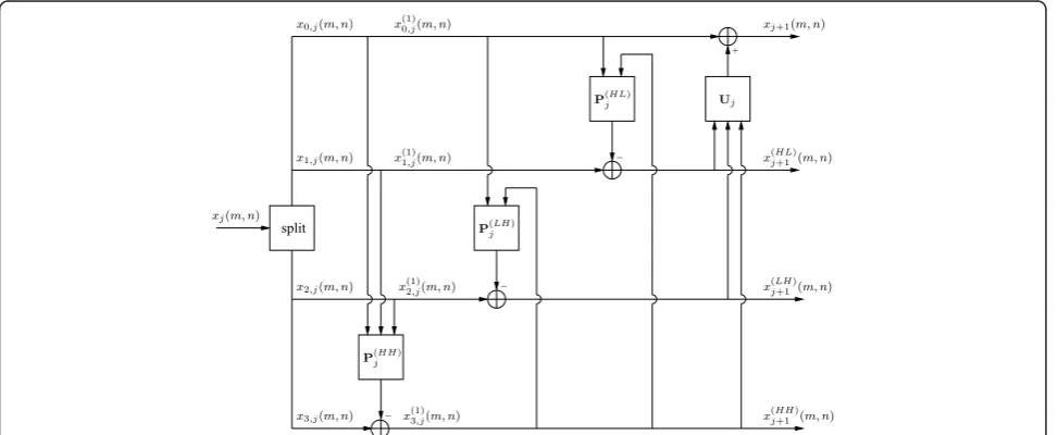
In this article, we consider a 2D NSLS composed of three prediction lifting steps followed by an update lift-ing step. The interest of this structure is two-fold. First, it allows us to reduce the number of lifting steps and rounding operations. A theoretical analysis has been conducted in [13] showing that NSLS improves the coding performance due to the reduction of round-ing effects. Furthermore, any separable prediction-update LS structure has its equivalent in this form [13,14]. The corresponding analysis structure is depicted in Figure 1.
Let x denote the digital image to be coded. At each resolution level j and each pixel location (m, n), its
approximation coefficient is denoted byxj(m, n) and the associated four polyphase components by x0,j(m, n) = xj (2m,2n),x1,j(m,n) =xj(2m,2n+1),x2,j(m,n) = xj(2m+1,2n), and x3,j(m,n) = xj(2m + 1, 2n + 1). Furthermore, we denote by P(jHH), Pj(LH), P(jHL), and Ujthe three predic-tion and update filters employed to generate the detail
coefficients x(j+1HH) oriented diagonally, x(j+1LH) oriented
vertically, x(j+1HL) oriented horizontally, and the
approxi-mation coefficientsxj+1. In accordance with Figure 1, let us introduce the following notation:
•For the first prediction step, the prediction multi-ple input, single output (MISO) filter P(jHH) can be seen as a sum of three single input, single output
(SISO) filters P(0,HHj ), P(1,HHj ), and P(2,HHj ) whose respec-tive inputs are the componentsx0,j,x1,jandx2,j.
•For the second (resp. third) prediction step, the prediction MISO filter P(jLH) (resp. P(jHL)) can be
seen as a sum of two SISO filters P(0,LHj ) and P(1,LHj )
(resp. P(0,HLj ) and P(1,HLj )) whose respective inputs are
the componentsx2,jand x(j+1HH) (resp.x1,jand x(j+1HH)).
•For the update step, the update MISO filter Ujcan be seen as a sum of three SISO filters U(jHL), U(jLH),
and U(jHH) whose respective inputs are the detail
coefficients x(j+1HL), x(j+1LH), and x(j+1HH).
Now, it is easy to derive the expressions of the result-ing coefficients in the 2Dz-transform domain.aIndeed,
split
−
−
−
+
P(HL)
j
P(LH)
j
P(HH)
j
xj(m, n)
x1,j(m, n)
x2,j(m, n)
x3,j(m, n)
x0,j(m, n)
x(1) 2,j(m, n)
xj+1(m, n)
x(HL)
j+1(m, n)
x(LH)
j+1(m, n)
x(HH)
j+1 (m, n) x(1)
0,j(m, n)
x(1) 1,j(m, n)
x(1) 3,j(m, n)
Uj
the z-transforms of the output coefficients can be expressed as follows:
Xj+1(HH)(z1,z2) =X3,j(z1,z2)− P0,j(HH)(z1,z2)X0,j(z1,z2) +P(HH)1,j (z1,z2)X1,j(z1,z2) +P(HH)2,j (z1,z2)X2,j(z1,z2),
(1)
X(LH)j+1(z1,z2) =X2,j(z1,z2)−P0,j(LH)(z1,z2)X0,j(z1,z2) +P(LH)1,j (z1,z2)X(HH)j+1 (z1,z2), (2)
X(HL)j+1(z1,z2) =X1,j(z1,z2)−
P(HL)0,j (z1,z2)X0,j(z1,z2) +P (HL) 1,j (z1,z2)X
(HH) j+1 (z1,z2)
, (3)
Xj+1(z1,z2) =X0,j(z1,z2) +U(HL)j (z1,z2)Xj+1(HL)(z1,z2) +U(LH)j (z1,z2)X(LH)j+1 (z1,z2) +U(HH)j (z1,z2)X
(HH) j+1 (z1,z2)
(4)
where, for every polyphase index i Î {0,1, 2} and orientationoÎ{HH, HL, LH},
Pi,j(o)(z1,z2) =
(k,l)∈P(o)
i,j
p(o)i,j(k,l)z− k 1z−
1
2 , and U
(o) j (z1,z2) =
(k,l)∈U(o)
j
u(o)j (k,l)z− k 1z−
l 2.
The set Pi(,oj) (resp. Uj(o)) and the coefficients p(i,oj)(k,l)
(resp. u(jo)(k,l)) denote the support and the weights of the three prediction filters (resp. of the update filter). Note that in Equations (1)-(4), we have introduced the rounding operations⌊.⌋in order to allow lossy-to-loss-less encoding of the coefficients [7]. Once the consid-ered NSLS structure has been defined, we will focus now on the optimization of its lifting operators.
2.2 Optimization methods
Since the detail coefficients are defined as prediction errors, the prediction operators are often optimized by minimizing the variance of the coefficients (i.e., theirℓ2 -norm) at each resolution level. The rounding operators being omitted, it is readily shown that the minimum variance predictors must satisfy the well-known Yule-Walker equations. For example, for the prediction vector
p(jHH), the normal equations read
E[x˜(jHH)(m,n)x˜(jHH)(m,n)T]p(jHH)=E[x3,j(m,n)x˜(jHH)(m,n)] (5)
where
• p(jHH)= (p(0,HHj ),p1,(HHj ),p(2,HHj ))T is the prediction vector, and, for every iÎ{0, 1, 2},
p(i,HHj )=
p(i,HHj )(k,l)
(k,l)∈Pi,j(HH)
,
• x˜(jHH)(m,n) = (x(0,HHj )(m,n),x(1,HHj )(m,n),x2,(HHj )(m,n))T is the reference vector with
x(i,HHj )(m,n) =xi,j(m−k,n−l)
(k,l)∈Pi,j(HH).
The other optimal prediction filters p(jHL) and p(jLH)
are obtained in a similar way.
Concerning the update filter, the conventional approach consists of optimizing its coefficients by minimizing the reconstruction error when the detail signal is canceled [20,38]. Recently, we have proposed a new optimization technique which aims at reducing the aliasing effects [36,37]. To this end, the update operator is optimized by minimizing the quadratic error between the approximation signal and the deci-mated version of the output of an ideal low-pass fil-ter:
˜
J(uj) =E xj+1(m,n)−yj+1(m,n)
2 =E ⎡ ⎢ ⎣ ⎛ ⎜ ⎝x0,j(m,n) +
o∈{HL,LH,HH}
(k,l)∈U(o)
j
u(jo)(k,l)x (o)
j+1(m−k,n−l)−yj+1(m,n)
⎞ ⎟ ⎠ 2⎤ ⎥ ⎦ (6)
where yj+1(m,n) =˜yj(2m, 2n) = (h∗xj)(2m, 2n).
Recall that the impulse response of the 2D ideal low-pass filter is defined in the spatial domain by:
∀(m,n)∈Z2, h(m,n) = 1 4sin c
mπ 2
sin cnπ 2
.(7)
Thus, the optimal update coefficients ujminimizing the criterion J˜ are solutions of the following linear sys-tem of equations:
E[xj+1(m,n)xj+1(m,n)T]uj=E[yj+1(m,n)xj+1(m,n)]−E[x0,j(m,n)xj+1(m,n)]
Where
• uj=
u(jo)(k,l)
T
(k,l)∈Uj(o),o∈{HL,LH,HH}
is the update
weight vector,
• xj+1(m,n) =
x(j+1o)(m−k,n−l)T (k,l)∈P(o)
i,j,o∈{HL,LH,HH}
is the reference vector containing the detail signals previously computed at thejth resolution level.
Now, we will introduce a novel twist in the optimiza-tion of the different filters: the use of anℓ1-based criter-ion in place of the usualℓ2-based measure.
3 From ℓ2to ℓ1 minimization 3.1 Motivation
∀x∈R, f(x;α,β) = β 2α 1 β e−
|x|
α β
(8)
where (z) =0+∞tz−1e−tdt is the Gamma function, a
> 0 is the scale parameter, andb> 0 is the shape para-meter. We should note that in the particular case when b= 2 (resp.b= 1), the GGD corresponds to the Gaus-sian distribution (resp. the Laplace one). The parameters aandbcan be easily estimated by using the maximum likelihood technique [42].
Let us now adopt this probabilistic GGD model for the detail coefficients generated by a lifting structure. More precisely, at each resolution leveljand orientation
o(oÎ {HL,LH,HH}), the wavelet coefficients xj(+1o)(m,n)
are viewed as realizations of random variable X(j+1o) with
probability distribution given by a GGD with parameters
α(o)
j+1 and β
(o)
j+1. Thus, this class of distributions leads us to the following sample estimate of the differential entropyhof the variable Xj(+1o)[11,43]:
h(X(j+1o))≈ ⎛ ⎜
⎝ 1
MjNj(αj(+1o))
β(o)
j+1 ln(2) ⎞ ⎟ ⎠ Mj m=1 Nj n=1 x(j+1o)(m,n)
β(o)
j+1
−log2 ⎛ ⎜ ⎜ ⎜ ⎜ ⎜ ⎜ ⎝
β(o) j+1
2α(o) j+1
⎛ ⎝1
β(o) j+1 ⎞ ⎠ ⎞ ⎟ ⎟ ⎟ ⎟ ⎟ ⎟ ⎠ (9)
where (Mj,Nj) corresponds to the dimensions of the subband x(j+1o).
Let
¯
x(j+1o)(m,n) 1≤m≤Mj
1≤n≤Nj
be the outputs of a uniform
quantizer with quantization stepqdriven with the
real-valued coefficients
x(j+1o)(m,n) 1≤m≤Mj
1≤n≤Nj
. The coefficients
X(j+1o) can be viewed as realizations of a random variable
X(j+1o) taking its values in {..., -2q, -q, 0,q, 2q, ...}. At high resolution, it was proved in [43] that the following
rela-tion holds between the discrete entropy X(j+1o) and the
differential entropyhof X(j+1o):
H(X(j+1o))≈h(Xj(+1o))−log2(q). (10)
Thus, from Equation (9), we see [44] that the entropy
H(X(j+1o)) of X(j+1o) is (up to a dividing factor and an addi-tive constant) approximaaddi-tively equal to:
Mj m=1 Nj n=1
x(j+1o)(m,n)β
(o) j+1
.
This shows that there exists a close link between the minimization of the entropy of the detail wavelet
coeffi-cients and the minimization of their β(o)j+1-norm. This
suggests in particular that most of the existing studies minimizing the ℓ2-norm of the detail signals aim at minimizing their entropy by assuming a Gaussian model.
Based on these results, we have analyzed the detail wavelet coefficients generated by the decomposition based on the lifting structure NSLS(2,2)-OPT-L2 described in Section 6. Figure 2 shows the distribution of each detail subband for the “einst” image when the prediction filters are optimized by minimizing the ℓ2 -norm of the detail coefficients. The maximum likelihood technique is used to estimate thebparameter.
It is important to note that the shape parameters of the resulting detail subbands are closer tob= 1 thanto
b= 2. Further experiments performed on a large dataset of imagesb have shown that the average ofbvalues are
−080 −60 −40 −20 0 20 40 60 80 100 0.01 0.02 0.03 0.04 0.05 0.06 0.07 0.08
−1200 −100 −80 −60 −40 −20 0 20 40 60 80 0.01 0.02 0.03 0.04 0.05 0.06 0.07 0.08
−080 −60 −40 −20 0 20 40 60 80 100 0.01 0.02 0.03 0.04 0.05 0.06 0.07 0.08
(a) (b) (c)
Figure 2 The GGD of the. (a) horizontal detail subband x(HL)
1 (β (HL)
1 = 1.07),(b): vertical detail subband x
(LH) 1 (β
(LH)
1 = 1.14), (c):
diagonal detail subbandx(HH)
1 (β
(HH)
closer to 1 (typical values range from 0.5 to 1.5). These observations suggest that minimizing theℓ1-norm may be more appropriate thanℓ2 minimization. In addition, the former approach has the advantage of producing sparse representations.
3.2ℓ1minimization technique
Instead of minimizing the ℓ2-norm of the detail
coeffi-cients x(j+1o) as done in [37], we propose in this section to optimize each of the prediction filters by minimizing the followingℓ1criterion:
∀o∈ {HL,LH,HH},∀i∈ {1, 2, 3}, J1(p
(o) j ) =
Mj m=1 Nj n=1
xi,j(m,n)−(p(jo)) T
˜
x(o) j (m,n)
(11)
wherexi,j(m,n) is the (i +1)thpolyphase component to
be predicted, x˜(jo)(m,n) is the reference vector
contain-ing the samples used in the prediction step, p(jo) is the
prediction operator vector to be optimized (Lwill subse-quently designate its length). Although the criterion in (11) is convex, a major difficulty that arises in solving this problem stems from the fact that the function to be minimized is not differentiable. Recently, several optimi-zation algorithms have been proposed to solve non-smooth minimization problems like (11). These problems have been traditionally addressed with linear programming [45]. Alternatively, a flexible class of prox-imal optimization algorithms has been developed and successfully employed in a number of applications. A survey on these proximal methods can be found in [46]. These methods are also closely related to augmented Lagrangian methods [47]. In our context, we have employed the Douglas-Rachford algorithm which is an efficient optimization tool for this problem [48].
3.2.1 The Douglas-Rachford algorithm
For minimizing the ℓ1 criterion, we will resort to the concept of proximity operators [49], which has been recognized as a fundamental tool in the recent convex optimization literature [50,51]. The necessary back-ground on convex analysis and proximity operators [52,53] is given in Appendix A.
Now, we recall that our minimization problem (11) aims at optimizing the prediction filters by minimizing the ℓ1-norm of the difference between the current pixel
xi,j and its predicted value. We note here that
xi,j=
xi,j(m,n)
1≤m≤Mj
1≤n≤Nj can be viewed as an element of
the Euclidean space RKj, whereKj=Mj×Nj. Thus, the
minimization problem (11) can be rewritten as:
∀o∈ {HL,LH,HH},∀i∈ {1, 2, 3}, min
z(o)
j ∈V
Mj m=1 Nj n=1
xi,j(m,n)−z(o)j (m,n) (12)
whereVis the vector space defined as
V=z(o)j =
z(o)j (m,n)
1≤m≤Mj
1≤n≤Nj
∈RKj|∃p(o) j ∈RL,
∀(m,n)∈ {1,. . .,Mj} × {1,. . .,Nj},z(o)j (m,n) = (p (o) j )Tx˜
(o) j (m,n)}.
Based on the definition of the indicator function ıV (see Appendix A), Problem (12) is equivalent to the fol-lowing minimization problem:
∀o∈ {HL,LH,HH},∀i∈ {1, 2, 3}, min
z(o)
j∈RKj
Mj m=1 Nj n=1
xi,j(m,n)−z(jo)(m,n)+ıV(z(jo)). (13)
Therefore, Problem (13) can be viewed as a minimiza-tion of a sum of two funcminimiza-tionsf1andf2 defined by:
f1(z(jo)) =||xi,j−z(jo)||1= Mj m=1 Nj n=1
xi,j(m,n)−zj(o)(m,n)(14)
f2(z(jo)) =ıV(z(jo)). (15)
In this case, the Douglas-Rachford algorithm can be applied to provide an appealing numerical solution to Problem (13) (see Appendix B).
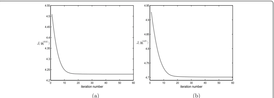
Although it is an iterative algorithm, we have observed experimentally that the convergence of the Douglas-Rachford algorithm is generally ensured after a small number of iterations (often between 30 et 60 iterations). As an example, we plot in Figure 3a (resp. 3b) the evo-lution of the criterion J1(p(0HH))(resp. J1(p(0LH))) w.r. t the iteration number for this algorithm.
Once the different terms involved in the iterative algo-rithm (33) are defined, this one can be applied and further extended to optimize all the prediction filters.
4 Global prediction error minimization technique
4.1 Motivation
Up to now, each prediction filter
p(jo)(o∈ {HL,LH,HH}) has been separately optimized by minimizing theℓ1-norm of the corresponding detail signal x(j+1o) which seems appropriate to determine p(jLH)
and p(jHL). However, it can be noticed from Figure 1
that the diagonal detail signal x(j+1HH) is also used through the second and the third prediction steps to compute the vertical and the horizontal detail signals respectively. Therefore, the solution p(jHH) resulting from the
pre-vious optimization method may be suboptimal. As a result, we propose to optimize the prediction filter
4.2 Optimization of the prediction filter p(jHH)
More precisely, instead of minimizing the ℓ1-norm of
x(j+1HH), the filter p(jHH) will be optimized by minimizing the sum of the ℓ1-norm of the three detail subbands
x(j+1o). To this respect, we will consider the minimization of the following weightedℓ1criterion:
Jw1(p
(HH)
j ) =
o∈{HL,LH,HH}
m,n κ(o)
j+1x (o)
j+1(m,n) (16)
where κj(+1o), o Î {HL, LH, HH}, are strictly positive
weighting terms.
Before focusing on the method employed to minimize the proposed criterion, we should first express Jw1 as a
function of the filter p(jHH) to be optimized.
Let
x(1)i,j (m,n)
i∈{0,1,2,3} be the four outputs obtained from xi,j(m,n)
i∈{0,1,2,3} following the first prediction step (see Figure 1). Although x(1)i,j (m,n) =xi,j(m,n) for
all iÎ{0, 1, 2}, the use of the superscript will make the
presentation below easier. Thus x(j+1o) can be expressed as:
x(o)j+1(m,n) =
i∈{0,1,2,3}
k,l h(o,1)i,j (k,l)x
(1) i,j(m−k,n−l)
=
i∈{0,1,2}
k,l h(o,1)i,j (k,l)x
(1)
i,j(m−k,n−l) +
k,l h(o,1)3,j (k,l)x
(1) 3,j(m−k,n−l)
(17)
where h(i,oj,1) is a filter which depends on the
predic-tion coefficients of p(jLH) and p(jHL).
Knowing that
x(1)3,j(m,n) =x3,j(m,n)−(p(jHH))Tx˜j(HH)(m,n) (18)
where x˜ (HH)
j (m,n) =
xi,j(m−r,n−s)
(r,s)∈Pj(HH)
i∈{0,1,2}
(Pj(HH)
is the support of the predictor p(jHH)), we thus obtain, after some simple calculations,
∀o∈ {HH,LH,HL}, x(o)j+1(m,n) =y(o,1)j (m,n)−(p(HH)j )Tx(0,1)
j (m,n) (19)
Where
y(o,1) j (m,n) =
i∈{0,1,2}
k,l
h(o,1) i,j (k,l)x
(1)
i,j(m−k,n−l) +
k,l
h(o,1)
3,j (k,l)x3,j(m−k,n−l), (20)
x(o,1)j (m,n) =
⎛
⎝
k,l
h(o,1)3,j (k,l)xi,j(m−k−r,n−l−s)
⎞ ⎠
(r,s)∈P(HH)
j i∈{0,1,2}
. (21)
Consequently, the proposed weighted ℓ1 criterion (Equation (16)) can be expressed as:
Jw1(p
(HH)
j ) =
o∈{HL,LH,HH}
m,n
κ(o) j+1
y(o,1)j (m,n)−(p(HH)j )Tx(o,1)j (m,n). (22)
It is worth noting that in practice, the determination
of yj(o,1)(m,n) and x(jo,1)(m,n) does not require to find
the explicit expressions of h(i,oj,1)and these signals can be
determined numerically as follows:
•The first term (resp. the second one) in the expres-sion of y(jo,1)(m,n) in Equation (20) can be found by
computing x(j+1o)(m,n) from the components
0 10 20 30 40 50 60
4.2 4.25 4.3 4.35 4.4 4.45 4.5 4.55 iteration number
J1(p(0HH))
0 10 20 30 40 50 60
4.7 4.75 4.8 4.85 4.9 4.95 iteration number
J1(p(0LH))
(a) (b)
Figure 3Convergence of the Douglas Rachford algorithm w.r.t the iteration number: (a) evolution of J
1(p
(HH)
0 ), (b) evolution of J1(p
J1(p
(LH)
0 ) while setting x (1)
3,j(m,n) = 0 (resp. while
set-ting x(1)i,j (m,n) = 0 for i Î {0,1,2} and
x(1)3,j(m,n) =x3,j(m,n)).
• The vector x(jo,1)(m,n) in Equation (21) can be found as follows. For eachiÎ {0,1,2}, the computation of its component k,lh(3,o,1)j (k,l)xi,j(m−k,n−l)
requires to compute x(j+1o)(m,n) by setting
x(1)3,j(m,n) =xi,j(m,n) and x(1)i,j(m,n) = 0 for i’ Î {0,1,2}.
The result of this operation has to be considered for dif-ferent shift values (r, s) (as can be seen in Equation (21)).
Once the different terms involved in the proposed weighted criterion in Equation (22) are defined (the con-stant values κj(+1o) are supposed to be known), we will focus now on its minimization. Indeed, unlike the pre-vious criterion (Equation 11), which consists only of an
ℓ1 term, the proposed criterion is a sum of three ℓ1 terms. To minimize such a criterion (22), one can still use the Douglas-Rachford algorithm through a formula-tion in a product space [46,54].
4.2.1 Douglas-Rachford algorithm in a product space
Consider theℓ1 minimization problem:
min
P(jHH)
o∈{H,L,LH,HH}
m,n
kj(+1o)yj(o,1)(m,n)−(p(jHH))Txj(o,1)(m,n) (23)
where κj(+1o),oÎ {HL,LH,HH}, are positive weights. Since the Douglas-Rachford algorithm described here-above is designed for the sum of two functions, we can reformulate (23) under this form in the 3-fold product space Hj
Hj=RKj×RKj×RKj. (24)
If we define the vector subspaceUas
U=Zj=
⎛ ⎜ ⎝
z(jHH,1)
z(jLH,1)
z(HL,1) j
⎞ ⎟
⎠∈Hj|∃p(jHH)∈R L
,∀o∈ {HH,LH,HL},
∀(m,n)∈ {1, 2,. . .,Mj} × {1, 2,. . .,Nj},z
(o,1)
j (m,n) = (p
(HH)
j )
T
x(jo,1)(m,n)
=Zj=
⎛ ⎜ ⎝
z(jHH,1)
z(LH,1) j
z(HL,1) j
⎞ ⎟
⎠∈Hj|∃p(jHH)∈R L
,∀(m,n)∈ {1, 2,. . .,Mj} × {1, 2,. . .,Nj},
Zj(m,n) =Xj(m,n)Tp(jHH)withXj(m,n) =
x(HH,1)
j (m,n),x
(LH,1)
j (m,n),x
(HL,1)
j (m,n)
!
,
(25)
the minimization problem (Equation 23) is equivalent to
min zj∈Hj
f3(zj) +f4(zj) (26)
where
f3(zj) =
o∈{HL,LH,HH}
m,n
κ(o) j+1y
(o,1)
j (m,n)−z (o,1) j (m,n)
f4(zj) =ıU(zj).
(27)
We are thus back to a problem involving two func-tions in a larger space, which is the product space Hj.
So, the Douglas-Rachford algorithm can be applied to solve our minimization problem (see Appendix C). Finally, once the prediction filter p(jHH) is optimized and
fixed, it can be noticed that the other prediction filters
p(jHL) and p(jLH) can be separately optimized by
mini-mizing J1(p
(HL)
j ) and J1(p
(LH)
j ) as explained in
Sec-tion 3. This is justified by the fact that the inputs of the filter p(jHL) (resp. p(jLH)) are independent of the output
of the filter p(jLH) (resp. p(jHL)).
5 Joint optimization method
5.1 Motivation
From Equations (20) and (21), it can be observed that
yj(o,1) and xj(o,1), which are used to optimize p(jHH),
depend on the coefficients of the prediction filters p(jHL)
and p(jLH). On the other hand, since pj(HL) and p(jLH)
use x(j+1HH) as reference signal in the second and the third prediction steps, their optimal values will depend
on the optimal prediction filter p(jHH). Thus, we
con-clude that the optimization of the filters (p(jHL), p(jLH))
depends on the optimization of the filter p(jHH) and vice-versa.
A joint optimization method can therefore be
pro-posed which iteratively optimizes the prediction filters
pj(HL), pj(HL), and p(jLH).
5.2 Proposed algorithms
While the optimization of the prediction filters p(jHL)
and p(jLH) is simple, the optimization of the prediction
filter p(jHH) is less obvious. Indeed, if we examine the
criterion Jw1, the immediate question that arises is:
which values of the weighting parameters will produce the sparsest decomposition?
A simple solution consists of setting all the weights
κ(o)
of the unweightedℓ1 criterion, which simply represents the sum of the ℓ1-norm of the three details subbands x(j+1o). In this case, the joint optimization problem is solved by applying the following simple iterative algo-rithm at each resolution levelj.
5.2.1 First proposed algorithm
➀ Initialize the iteration numberitto 0.
•Optimize separately the three prediction filters as explained in Section 3. The resulting filters will be denoted respectively by p(jHH,0), p(jLH,0),
and p(jHL,0).
•Compute the resulting global unweighted pre-diction error (i.e., the sum of theℓ1-norm of the three resulting details subbands).
➁ forit= 1,2,3,
• Set p(jLH)=p(jLH,it−1),p(jHL)=p(jHL,it−1), and
optimize P(jHH) by minimizing Jw1(p
(HH)
j )
(while setting κj(+1o)= 1). Let p(jHH,it) be the new
optimal filter at iterationit.
• Set p(jHH)=pj(HH,it), and optimize P(jLH) by
minimizing J1(p(0LH)). Let p(jLH,it) be the new optimal filter.
• Set p(jHH)=pj(HH,it), and optimize P(jHL) by
minimizing J1(p
(HL)
j ). Let p
(HL,it)
j be the new
optimal filter.
Once the prediction filters are optimized, the update filter is finally optimized as explained in Section 2. How-ever, in practice, once all the filters are optimized and the decomposition is performed, the different generated
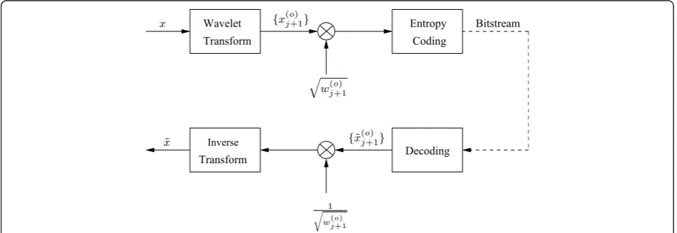
wavelet subbands x(j+1o) are weighted before the entropy encoding (using JPEG2000 encoder) in order to obtain a distortion in the spatial domain which is very close to the distortion in the wavelet domain.
More precisely, as we can see in Figure 4, each
wave-let subband is multiplied by "w(j+1o), where w(j+1o)
repre-sents the weight corresponding to x(j+1o). Generally, these weights are computed based on the wavelet filters used for the reconstruction process as indicated in [55,56]. A simple weight computation procedure based on the fol-lowing assumption can be used. As shown in [55], if the error signal in a subband (i.e., the quantization noise) is white and uncorrelated to the other subband errors, the reconstruction distortion in the spatial domain is a weighted sum of the distortion in each wavelet subband. Therefore, for each subband x(j+1o), a white Gaussian
noise of variance (σj(+1o))2 is firstly added while keeping the remaining subbands noiseless. Then, the resulting distortion in the spatial domain Dˆs is evaluated by
tak-ing the inverse transform. Finally, the correspondtak-ing subband weight can be estimated as follows:
w(j+1o) = Dˆs×4
j+1
(σj(+1o))2
. (28)
This weighting step is very important since standard bit allocation algorithms assume that the quadratic dis-tortion in the wavelet domain is equal to that in the spatial domain, which is not true in the case of biortho-gonal wavelets [55]. Therefore, the filters resulting from
the first choice of κj(+1o) are suboptimal in the sense that they do not take into account the weighting procedure.
Coding Wavelet
Transform
Transform
Inverse
Decoding
Bitstream Entropy
{x(o)j+1}
{˜x(o)j+1}
w(o)j+1
1
w(jo+1)
x
˜
x
For this reason, it has been noticed on some experi-ments (as it can be seen in Section 6) that the basic optimization technique does not achieve the best coding performances.
Thus, a more judicious choice of κj(+1o) should take into account the weighting procedure applied to the wavelet coefficients before the entropy encoding process. Furthermore, if in the general formula in Equation (9), we consider the case of βj(+1o)= 1, the differential entropy
of X(j+1o) multiplied by "w(j+1o) becomes:
1
MjNjαj(+1o)ln(2) Mj m=1 Nj n=1
x(j+1o)(m,n)+ log2
2αj(+1o)
"
w(j+1o)
(29)
where αj(+1o) can be estimated by using a classical maxi-mum likelihood estimate. Thus, it can be observed from Equation (29) that the first term of the resulting entropy, which corresponds to a weighted ℓ1-norm of
x(j+1o), is inversely proportional to α(j+1o). Consequently, in order to obtain a criterion (Equation 16) that results in a good approximation of the entropy (29), a more rea-sonable choice of κj(+1o) will be as follows:
κ(o)
j+1= 1
α(o)
j+1
. (30)
Since the resulting entropy of each subband uses weights which also depend on the prediction filters (as mentioned above), we propose an iterative algorithm that alternates between optimizing all the filters and redefining the weights. This algorithm, which is per-formed for each resolution levelj, is as follows.
5.2.2 Second proposed algorithm
➀ Initialize the iteration numberitto 0.
•Optimize separately the three prediction filters as explained in Section 3. The resulting filters will be denoted respectively by p(jHH,0), p(jLH,0),
and p(jHL,0).
•Optimize the update filter (as explained in Sec-tion 2).
•Compute the weights w(j+1o,0) of each detail
sub-band as well as the constant values κj(+1o,0). ➁ forit =1,2,3,...
• Set p(jLH)=p(jLH,it−1),p(jHL)=p(jHL,it−1), and
optimize P(jHH) by minimizing Jw1(p
(HH)
j ). Let p(jHH,it) be the new optimal filter.
• Set p(jHH)=pj(HH,it), and optimize P(jLH) by
minimizing J1(p
(LH)
j ). Let p
(LH,it)
j be the new
optimal filter.
• Set p(jHH)=pj(HH,it), and optimize P(jHL) by
minimizing J1(p(jHL)). Let p(jHL,it) be the new
optimal filter.
•Optimize the update filter (as explained in Sec-tion 2).
• Compute the new weights w(j+1o,it) as well as
κ(o,it)
j+1 .
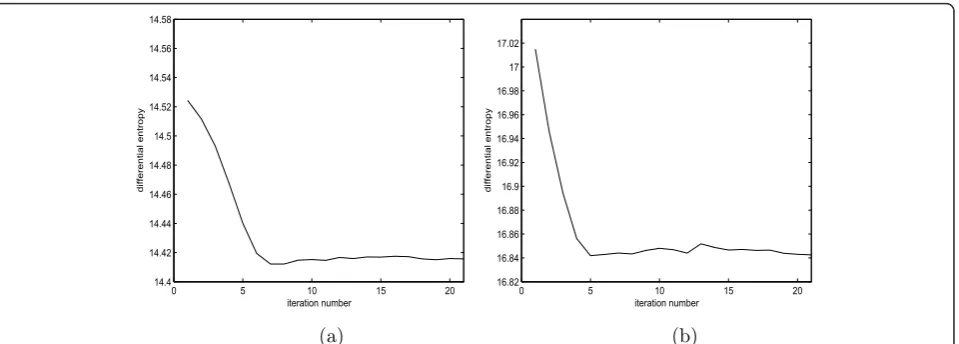
Let us now make some observations concerning the convergence of the proposed algorithm. Since the goal of the second weighting procedure is to better approxi-mate the entropy, we have computed at the end of each iteration numberitthe differential entropy of the three resulting details subbands. More precisely, the evaluated criterion, obtained from Equation (29) by setting
α(o)
j+1= 1
κ(o)
j+1
and performing the sum over the three
details subbands, is given by:
o∈{HL,LH,HH} ⎛ ⎜
⎝ κ
(o,it) j+1 MjNjln(2)
Mj m=1 Nj n=1
|x(o)j+1(m,n)|+ log2
⎛ ⎜ ⎝2
"
w(o,it)j+1
κ(o,it) j+1 ⎞ ⎟ ⎠ ⎞ ⎟ ⎠. (31)
Figure 5 illustrates the evolution of this criterion w.r.t the iteration number of the algorithm. It can be noticed that the decrease of the criterion is mainly achieved dur-ing the early iterations (about after 7 iterations).
6 Experimental results
Simulations were carried out on two kinds of still images originally quantized over 8 bpp which are either single views or stereoscopic ones. A large dataset com-posed of 50 still imagesband 50 stereo imageschas been considered. The gain related to the optimization of the NSLS operators, using different minimization criteria, was evaluated in these contexts. In order to show the benefits of the proposed ℓ1 optimization criterion, we provide the results for the following decompositions car-ried out over three resolution levels:
•The first one is the LS corresponding to the 5/3 transform, also known as the (2,2) wavelet transform [7]. In the following, this method will be designated by NSLS(2,2).
by minimizing the ℓ2-norm of the detail coefficients whereas the update filter is optimized by minimizing the reconstruction error. This optimization method will be designated by NSLS(2,2)-OPT-GM.
• The third approach corresponds to our previous method presented recently in [37]. While the predic-tion filters are optimized in the same way as the sec-ond method, the update filter is optimized by minimizing the difference between the approxima-tion signal and the decimated version of the output of an ideal low-pass filter. We emphasize here that the prediction filters are optimized separately. This method will be denoted by NSLS(2,2)-OPT-L2.
•The fourth method modifies the optimization stage of the prediction filters by using the ℓ1-norm instead of the ℓ2-norm. The optimization of the update filter is similar to the technique used in the third method. In what follows, this method will be designated by NSLS(2,2)-OPT-L1.
•The fifth method consists ofjointly optimizing the prediction filters by using the proposed weighted ℓ2
minimization technique where the weights κj(+1o) are
set to 1
α(o)
j+1
. The optimization of the update filter is
similar to the technique used in the third and fourth methods. This optimization method will be desig-nated by NSLS(2,2)-OPT-WL1. We have also tested this optimization method when the weights κj(+1o) are set to 1. In this case, the method will be denoted by
NSLS(2,2)-OPT-WL1 (κj(+1o)= 1).
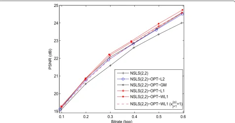
Figures 6 and 7 show the scalability in quality of the reconstruction procedure by providing the variations of the PSNR versus the bitrate for the images“castle” and
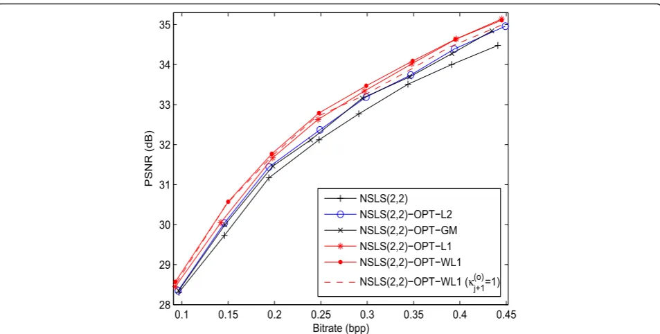
“straw” using JPEG2000 as entropy codec. A more exhaustive evaluation was also performed by applying the different methods to 50 still imagesb. The average
PSNR per-image is illustrated in Figure 8.
These plots show that NSLS(2,2)-OPT-L2 outperforms NSLS(2,2) by 0.1-0.5 dB. It can also be noticed that NSLS(2,2)-OPT-L2 and NSLS(2,2)-OPT-GM perform similarly in terms of quality of reconstruction. An improvement of 0.1-0.3 dB is obtained by using the ℓ1 minimization technique instead of theℓ2 one. Finally,
the jointoptimization technique (NSLS(2,2)-OPT-WL1)
outperforms theseparateoptimization technique (NSLS (2,2)-OPT-L1) and improves the PSNR by 0.1-0.2 dB. The gain becomes more important (up to 0.55 dB) when compared with NSLS(2,2)-OPT-L2. It is important to note here that setting the weights κj(+1o) to 1 (NSLS
(2,2)-OPT-WL1 (κj(+1o)= 1)) can yield to a degradation of about 0.1-0.25 dB compared with NSLS(2,2)-OPT-WL1 on some images.
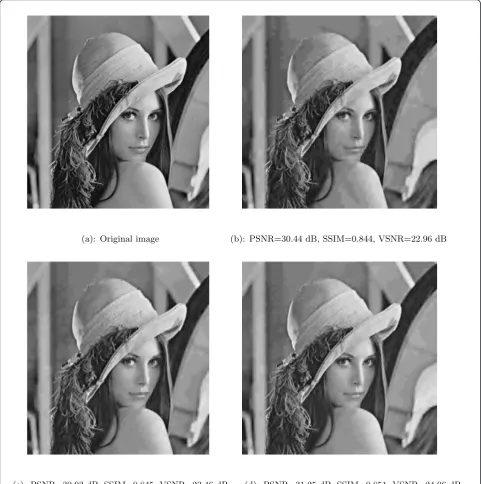
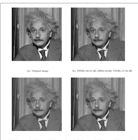
Figures 9 and 10 display the reconstructed images of
“lena” and “einst”. In addition to PSNR and SSIM metrics, the quality ofthe reconstructed images are also compared in terms of VSNR (Visual Signal-to-Noise ratio) which was found to be an efficient metric for quantifying the visual fidelity of natural images [57]: it is based on physical luminances and visual angle (rather than on digital pixel values and pixel-based dimensions) to accommodate different viewing conditions. It can be observed that the weightedℓ1 minimization technique significantly improves the visual quality of reconstruc-tion. The difference in VSNR (resp. PSNR) between NSLS(2,2)-OPT-L2 and NSLS(2,2)-OPT-WL1 ranges from 0.35 dB to 0.6 dB (resp. 0.25 dB to 0.3 dB). Com-paring Figure 9c (resp. Figure 10c) with Figure 9d (resp. Figure 10d), the visual improvement achieved by our
0 5 10 15 20
14.4 14.42 14.44 14.46 14.48 14.5 14.52 14.54 14.56 14.58
iteration number
differential entropy
0 5 10 15 20
16.82 16.84 16.86 16.88 16.9 16.92 16.94 16.96 16.98 17 17.02
iteration number
differential entropy
(a) (b)
method can be mainly seen in the hat and face of Lena (resp. in Einstein’s face).
The second part of the experiments is concerned with stereo images. Most of the existing studies in this field rely on disparity compensation techniques [58,59]. The basic principles involved in this technique first consists
of estimating the disparity map. Then, one image is con-sidered as a reference image and the other is predicted in order to generate a prediction error referred to as a residual image. Finally, the disparity field, the reference image and the residual one are encoded [58,60]. In this context, Moellenhoff and Maier [61] analyzed the
0.1 0.2 0.3 0.4 0.5 0.6
27 28 29 30 31 32 33 34 35
Bitrate (bpp)
PSNR (dB)
NSLS(2,2)
NSLS(2,2)−OPT−L2 NSLS(2,2)−OPT−GM NSLS(2,2)−OPT−L1 NSLS(2,2)−OPT−WL1 NSLS(2,2)−OPT−WL1 (κj+1(o)=1)
Figure 6PSNR (in dB) versus the bitrate (bpp) after JPEG2000 progressive encoding for the“castle”image.
0.1 0.2 0.3 0.4 0.5 0.6
19 20 21 22 23 24 25
Bitrate (bpp)
PSNR (dB)
NSLS(2,2)
NSLS(2,2)−OPT−L2 NSLS(2,2)−OPT−GM NSLS(2,2)−OPT−L1 NSLS(2,2)−OPT−WL1 NSLS(2,2)−OPT−WL1 (κj+1(o)=1)
characteristics of the residual image and proved that such images have properties different from natural images. This suggests that transforms that work well for natural images may not be as well-suited for residual images. For this reason, we also proposed to apply these optimization methods for encoding the reference image and the residual one. The resulting rate-distortion curves for the “white house” and “pentagon” stereo images are illustrated in Figures 11 and 12. A more exhaustive evaluation was also performed by applying the different methods to 50 stereo imagesc. Theaverage
PSNR per-image is illustrated in Figure 13. Figure 14 displays the reconstructed target image of the “ penta-gon” stereo pair. It can be observed that the proposed
jointoptimization method leads to an improvement of
0.35 dB (resp. 0.016) in VSNR (resp. SSIM) compared with the decomposition in which the prediction filters are optimizedseparately. For instance, it can be noticed that the edges of the pentagon’s building as well as the roads are better reconstructed in Figure 14d.
For completeness, the performance of the proposed method (NSLS(2,2)-OPT-WL1) has also been compared with the 9/7 transform retained for the lossy mode of JPEG2000 standard. Table 1 shows the performance of the latter methods in terms of PSNR, SSIM, and VSNR. Since the human eye cannot always distinguish the sub-jective image quality at middle and high bitrate, the results were restricted to the lower bitrate values.
While the proposed method is less performant in terms of PSNR than the 9/7 transform for some images, it can be noticed from Table 1 that better results are obtained in terms of perceptual quality. For instance, Figures 15 and 16 illustrate some reconstructed images. It can be observed that the proposed method (NSLS (2,2)-OPT-WL1) achieves a gain of about 0.2-0.4 dB (resp. 0.01-0.013) in terms of VSNR (resp. SSIM). Furthermore, Figures 17 and 18 display the recon-structed target image for the stereo image pairs“shrub” and“spot5”. While NSLS(2,2)-OPT-WL1 and 9/7 trans-form show similar visual quality for the “spot5” pair, the proposed method leads to better quality of reconstruc-tion than the 9/7 transform for the “shrub” stereo images.
Before concluding the article, let us now study the complexity of the proposed sparsity criteria for the opti-mization of the prediction filters. Table 2 gives the itera-tion number and the execuitera-tion time for the ℓ1 and weightedℓ1 minimization techniques when considering different image sizes. These results have been obtained with a Matlab implementation on an Intel Core 2 (2.93 GHz) architecture. It is clear that the execution time increases with the image size. Furthermore, we note that theℓ1 minimization technique is very fast whereas the weightedℓ1 technique needs an additional time of about 0.3-2.6 seconds. This increase is due to the fact that the algorithm is reformulated in a three-fold product space
0.1 0.2 0.3 0.4 0.5 0.6
19 20 21 22 23 24 25
Bitrate (bpp)
PSNR (dB)
NSLS(2,2)
NSLS(2,2)−OPT−L2 NSLS(2,2)−OPT−GM NSLS(2,2)−OPT−L1 NSLS(2,2)−OPT−WL1 NSLS(2,2)−OPT−WL1 (κj+1(o)=1)
as explained in Section 4.2. However, since the Douglas-Rachford algorithm in a product space has some blocks which can be implemented in a parallel way, the com-plexity can be reduced significantly (up to three times) when performing an appropriate implementation on a multicore architecture. These results as well as the good compression performance in terms of reconstruction quality confirm the effectiveness of the proposed spar-sity criteria.
7 Conclusion
In this article, we have studied different optimization techniques for the design of filters in a NSLS structure. A new criterion has been presented for the optimization of the prediction filters in this context. The idea consists
of jointly optimizing these filters by minimizing
itera-tively a weighted ℓ1 criterion. Experimental results car-ried out on still images and stereo images pair have illustrated the benefits which can be drawn from the (a): Original image (b): PSNR=30.44 dB, SSIM=0.844, VSNR=22.96 dB
(c): PSNR=30.93 dB, SSIM=0.845, VSNR=23.46 dB (d): PSNR=31.25 dB, SSIM=0.851, VSNR=24.06 dB
proposed optimization technique. In future study, we plan to extend this optimization method to LS with more than two stages like the P-U-P and P-U-P-U structures.
Appendix
A Some background on convex optimization
The main definitions which will be useful to understand our optimization algorithms are briefly summarized
below:
• ℝK
is the usual K-dimensional Euclidean space with norm ||.||.
•The distance function to a nonempty setC⊂ℝKis defined by
∀x∈RK, dC(x) = inf
y∈C||x−y||.
(a): Original image (b): PSNR=28.55 dB, SSIM=0.648, VSNR=17.82 dB
(c): PSNR=28.94 dB, SSIM=0.649, VSNR=18.24 dB (d): PSNR=29.12 dB, SSIM=0.654, VSNR=18.62 dB
•The projection of xÎ ℝKonto a nonempty closed convex set C ⊂ ℝK is the unique point PC(x) Î C such thatdC(x) = ||x- PC(x)||.
•The indicator function ofCis given by
∀x∈RK, ıC(x) = #
0 if x ∈C,
+∞ otherwise. (32)
•Γ0(ℝK) is the class of functions fromℝKto ] -∞, +
∞] which are lower semi-continuous, convex, and not identically equal to +∞.
• The proximity operator of f Î Γ0(ℝK) is
proxf :RK→RK:x→arg miny∈RKf(y) + 1 2||x−y||
2. It is
important to note that the proximity operator
0.1 0.15 0.2 0.25 0.3 0.35 0.4 0.45
28 29 30 31 32 33 34 35
Bitrate (bpp)
PSNR (dB)
NSLS(2,2) NSLS(2,2)−OPT−L2 NSLS(2,2)−OPT−GM NSLS(2,2)−OPT−L1 NSLS(2,2)−OPT−WL1 NSLS(2,2)−OPT−WL1 (κj+1(o)=1)
Figure 11PSNR (in dB) versus the bitrate (bpp) after JPEG2000 progressive encoding for the“white house”stereo images.
0.1 0.15 0.2 0.25 0.3 0.35 0.4 0.45
25 25.5 26 26.5 27 27.5 28 28.5 29
Bitrate (bpp)
PSNR (dB)
NSLS(2,2)
NSLS(2,2)−OPT−L2 NSLS(2,2)−OPT−GM NSLS(2,2)−OPT−L1 NSLS(2,2)−OPT−WL1 NSLS(2,2)−OPT−WL1 (κj+1(o)=1)
0.1 0.15 0.2 0.25 0.3 0.35 0.4 0.45 28
29 30 31 32 33 34
Bitrate (bpp)
PSNR (dB)
NSLS(2,2)
NSLS(2,2)−OPT−L2 NSLS(2,2)−OPT−GM NSLS(2,2)−OPT−L1 NSLS(2,2)−OPT−WL1 NSLS(2,2)−OPT−WL1 (κj+1(o)=1)
Figure 13Average PSNR (in dB) computed over 50 stereo images versus the bitrate (in bpp) after JPEG2000 progressive encoding.
(a): Original image (b): PSNR=26.44 dB, SSIM=0.693, VSNR=12.17 dB
(c): PSNR=26.56 dB, SSIM=0.691, VSNR=12.49 dB (d): PSNR=26.90 dB, SSIM=0.697, VSNR=13.06 dB
generalizes the notion of a projection operator onto a closed convex setCin the sense that proxıC =PC,
and it moreover possesses most of its attractive properties [49] that make it particularly well-suited for designing iterative minimization algorithms.
B The Douglas Rachford algorithm
The solution of the Problem (13) (which is the sum of the two functionsf1 andf2) is obtained by the following iterative algorithm:
Sett(j,0o)∈RKj,γ >0,λ∈]0, 2[, and,
fork= 0, 1, 2,. . .
z(j,ok)= proxγf2t
(o)
j,k
tj(,ok)+1=t(j,ok)+λ(proxγf1(2z
(o)
j,k −t
(o)
j,k)−z
(o)
j,k).
(33)
An important feature of this algorithm is that it pro-ceeds by splitting, in the sense that the functionsf1and
f2are dealt with in separate steps: in the first step, only
functionf2 is required to obtain z
(o)
j,k and, in the second Table 1 Performance of the proposed method vs the 9/7 transform
0.05 bpp 0.1 bpp 0.15 bpp 0.2 bpp
NSLS(2,2)-OPT-WL1 9/7 NSLS (2,2)-OPT-WL1 9/7 NSLS (2,2)-OPT-WL1 9/7 NSLS (2,2)-OPT-WL1 9/7
PSNR 27.85 27.75 30.25 30.31 31.23 31.35 31.76 31.92
elaine SSIM 0.669 0.659 0.716 0.715 0.739 0.739 0.754 0.756
VSNR 18.44 18.09 23.10 23.05 25.60 25.50 27.28 27.42
PSNR 25.10 25.09 27.08 27.18 28.36 28.51 29.51 29.58
castle SSIM 0.725 0.712 0.790 0.780 0.825 0.821 0.855 0.851
VSNR 17.54 17.22 21.55 21.10 23.74 23.40 25.80 25.32
PSNR 27.51 27.58 29.12 29.24 29.92 30.12 30.50 30.70
einst SSIM 0.603 0.601 0.654 0.655 0.687 0.689 0.710 0.715
VSNR 15.33 15.25 18.62 18.71 20.37 20.47 21.59 21.94
PSNR 26.70 26.68 29.59 29.56 31.25 31.47 32.70 32.90
lena SSIM 0.747 0.734 0.818 0.808 0.851 0.850 0.871 0.873
VSNR 15.94 15.73 20.56 20.18 24.06 23.95 26.12 26.15
PSNR 26.51 26.43 29.81 30.33 31.84 32.63 33.61 34.44
cameraman SSIM 0.783 0.774 0.847 0.842 0.887 0.892 0.914 0.915
VSNR 16.74 16.34 21.73 21.66 24.94 25.70 27.75 28.34
PSNR 24.65 24.55 26.82 26.86 28.43 28.54 29.52 29.74
boat SSIM 0.675 0.661 0.753 0.746 0.806 0.802 0.837 0.836
VSNR 13.41 13.03 17.14 16.89 20.24 19.76 22.19 21.89
PSNR 25.75 25.50 29.24 29.17 30.88 31.16 31.12 32.38
peppers SSIM 0.720 0.705 0.789 0.778 0.818 0.815 0.834 0.832
VSNR 16.00 15.51 21.87 21.19 25.18 25.00 27.22 27.09
PSNR 24.19 23.84 30.66 29.88 33.99 33.10 36.13 35.82
plane SSIM 0.809 0.754 0.890 0.871 0.917 0.903 0.931 0.921
VSNR 9.48 7.72 17.73 15.51 21.28 20.30 24.68 24.12
PSNR 24.88 24.72 27.67 27.73 29.24 29.46 30.45 30.65
average SSIM 0.647 0.633 0.727 0.720 0.773 0.771 0.803 0.802
VSNR 14.50 13.98 18.90 18.62 21.77 21.71 23.90 23.85
Theaverageevaluation was computed over 50 still images.
The values in bold have been used to identify the method achieving the best coding performance.
Table 2 Computation time (s) of the sparse optimization methods for the design of each prediction filter
Plane Girl Boat Cameraman
256 × 256 256 × 256 512 × 512 512 × 512
it Time (s) it time(s) it time(s) it time(s)
ℓ1criterion:p(HL)
0 22 0.09 27 0.09 30 0.38 60 0.81
ℓ1criterion:p(LH)
0 55 0.15 28 0.09 31 0.39 100 1.13
weightedℓ1criterion:p(HH)
step, only function f 1 is involved to obtain t
(o)
j,k+1. Furthermore, it can be seen that the algorithm requires to compute two proximity operators proxγf1, and
proxγf2 at each iteration. One can find in [46]
closed-form expression of the proximity operator of various
functions in Γ0(ℝ). In our case, the proximity operator ofgf1 is given by the soft-thresholding rule:
∀t(j,ok)∈RKj, prox
γf1(t
(o)
j,k) =
π(o)
j,k(m,n)
1≤m≤Mj
1≤n≤Nj
(34) (a): PSNR=26.68 dB, SSIM=0.734, VSNR=15.73 dB (b): PSNR=26.70 dB, SSIM=0.747, VSNR=15.94 dB
Figure 15Zoom applied on the reconstructed“lena”image at 0.05 bpp using: (a) 9/7 transform (b) NSLS(2,2)-OPT-WL1.
(a): PSNR=29.56 dB, SSIM=0.808, VSNR=20.18 dB (b): PSNR=29.59 dB, SSIM=0.818, VSNR=20.56 dB