Volume 2007, Article ID 45321,17pages doi:10.1155/2007/45321
Research Article
Calculation Scheme Based on a Weighted Primitive:
Application to Image Processing Transforms
Mar´ıa Teresa Signes Pont, Juan Manuel Garc´ıa Chamizo, Higinio Mora Mora, and Gregorio de Miguel Casado
Departamento de Tecnolog´ıa Inform´atica y Computaci´on, Universidad de Alicante, 03690 San Vicente del Raspeig, 03071 Alicante, Spain
Received 29 September 2006; Accepted 6 March 2007
Recommended by Nicola Mastronardi
This paper presents a method to improve the calculation of functions which specially demand a great amount of computing resources. The method is based on the choice of a weighted primitive which enables the calculation of function values under the scope of a recursive operation. When tackling the design level, the method shows suitable for developing a processor which achieves a satisfying trade-offbetween time delay, area costs, and stability. The method is particularly suitable for the mathe-matical transforms used in signal processing applications. A generic calculation scheme is developed for the discrete fast Fourier transform (DFT) and then applied to other integral transforms such as the discrete Hartley transform (DHT), the discrete co-sine transform (DCT), and the discrete co-sine transform (DST). Some comparisons with other well-known proposals are also provided.
Copyright © 2007 Mar´ıa Teresa Signes Pont et al. This is an open access article distributed under the Creative Commons Attribution License, which permits unrestricted use, distribution, and reproduction in any medium, provided the original work is properly cited.
1. INTRODUCTION
Mathematical notation aside, the motivation behind inte-gral transforms is easy to understand. There are many classes of problems that are extremely difficult to solve or, at least, quite unwieldy from the algebraic standpoint in their origi-nal domains. An integral transform maps an equation from its original domain (time or space domain) into another domain (frequency domain). Manipulating and solving the equation in the target domain is, ideally, easier than ma-nipulating and solving it in the original domain. The solu-tion is then mapped back into the original domain. Integral transforms work because they are based upon the concept of spectral factorization over orthonormal bases. Equation (1) shows the generic formulation of a discrete integral trans-form where f(x), 0≤x < N, andF(u), 0≤u < N, are the original and the transformed sequences, respectively. Both have N = 2n values, n ∈ N andT(x,u) is the kernel of the transform
F(u)=
N−1 x=0
T(x,u)f(x). (1)
The inverse transform can be defined in a similar way. Table 1shows some integral transforms (j=√−1 as usual).
Table1: Some integral transforms.
Transform KernelT(x,u) Remarks
Fourier 1
Nexp
−2jπux
N
Trigonometric kernel
Hartley cos 2πux
N
+ sin
2πux
N
Trigonometric kernel
Cosine e(k) cos(2x+ 1)πu 2N
Trigonometric kernel
withe(0)=√1 2,
e(k)=1, 0< k < N
Sine e(k) sin(2x+ 1)πu 2N
Trigonometric kernel
withe(0)=√1 2,
e(k)=1, 0< k < N
have an easier control because of their regular structure based on a constant indexation through all the stages. This allows parallel data processing by a column of processors with a fixed interconnecting net [12,13].
The Hartley transform is a Fourier-related transform which was introduced in 1942 by Hartley [14] and is very similar to the discrete Fourier transform (DFT), with analo-gous applications in signal processing and related fields. Its main distinction from the DFT is that it transforms real in-puts into real outin-puts, with no intrinsic involvement of com-plex numbers. The discrete Hartley transform (DHT) ana-logue of the Cooley-Tukey algorithm is commonly known as the fast Hartley transform (FHT) algorithm, and was first de-scribed in 1984 by Bracewell [15–17]. The transform can be interpreted as the multiplication of the vector (x0,. . .,xN−1) by anN×Nmatrix; therefore, the discrete Hartley transform is a linear operator. The matrix is invertible and the DHT is its own inverse up to an overall scale factor. This FHT al-gorithm, at least when applied to power-of-two sizesN, is the subject of a patent issued in 1987 to the University of Stanford. The University of Stanford placed this patent in the public domain in 1994 [18]. The DHT algorithms are typi-cally slightly less efficient (in terms of the number of floating-point operations) than the corresponding FFT specialized for real inputs or outputs [19,20]. The latter authors published the algorithm which achieves the lowest operation count for the DHT of power-of-two sizes by employing a split-radix al-gorithm, similar to that of the FFT. This scheme splits a DHT of lengthN into a DHT of lengthN/2 and two real-input DFTs (not DHTs) of lengthN/4. A priori, since the FHT and the real-input FFT algorithms have similar computational structures, none of them appears to have a substantial speed advantage [21]. As a practical matter, highly optimized real-input FFT libraries are available from many sources whereas highly optimized DHT libraries are less common. On the other hand, the redundant computations in FFTs due to real inputs are much more difficult to eliminate for large prime
N, despite the existence ofO(N·log2N) complex-data al-gorithms for that cases. This is because the redundancies are
hidden behind intricate permutations and/or phase rotations in those algorithms. In contrast, a standard prime-size FFT algorithm such as Rader’s algorithm can be directly applied to the DHT of real data for roughly a factor of two less com-putation than that of the equivalent complex FFT. This DHT approach currently appears to be the only way known to ob-tain such factor-of-two savings for large prime-size FFTs of real data [22]. A detailed analysis of the computational cost and specially of the numerical stability constants for DHT of types I–IV and the related matrix algebras is presented by Arico et al. [23]. The authors prove that any of these DHTs of lengthN =2t can be factorized by means of a divide–and– conquer strategy into a product of sparse, orthogonal matri-ces where in this context sparse means at most two nonzero entries per row and column. The sparsity joint with orthog-onality of the matrix factors is the key for proving that these new algorithms have low arithmetic costs and an excellent normwise numerical stability.
DCT is often used in signal and image processing, es-pecially for lossy data compression, because it has a strong “energy compaction” property: most of the signal informa-tion tends to be concentrated in a few low-frequency com-ponents of the DCT [24,25]. For example, the DCT is used in JPEG image compression, MJPEG, MPEG [26], and DV video compression. The DCT is also widely employed in solv-ing partial differential equations by spectral methods [27] and fast DCT algorithms are used in Chebyshev approxima-tion of arbitrary funcapproxima-tions by series of Chebyshev polynomi-als [28]. Although the direct application of these formulas would requireO(N2) operations, it is possible to compute them with a complexity of onlyO(N·log2N) by factoriz-ing the computation in the same way as in the fast Fourier transform (FFT). One can also compute DCTs via FFTs com-bined withO(N) pre- and post-processing steps. In princi-ple, the most efficient algorithms are usually those that are directly specialized for the DCT [29,30]. For example, par-ticular DCT algorithms resemble to have a widespread use for transforms of small, fixed sizes such as the 8×8 DCT used in JPEG compression, or the small DCTs (or MDCTs) typi-cally used in audio compression. Reduced code size may also be a reason for using a specialized DCT for embedded-device applications. However, even specialized DCT algorithms are typically closely related to FFT algorithms [22]. Therefore, any improvement in algorithms for one transform will the-oretically lead to immediate gains for the other transforms too [31]. On the other hand, highly optimized FFT programs are widely available. Thus, in practice it is often easier to ob-tain high performance for generalized lengths ofNwith FFT-based algorithms. Performance on modern hardware is typ-ically not simply dominated by arithmetic counts and opti-mization requires substantial engineering effort.
Table2: Definition of the operation⊕fork=1.
a⊕b 01=1 10=00=0 11= −1
01=1 α+β α α−β
10=00=0 β 0 −β
11= −1 −α+β −α −α−β
The applications of DST are similar to those for DCT as well as its computational complexity. The problem of reflecting boundary conditions (BCs) for blurring models that lead to fast algorithms for both deblurring and detecting the regu-larization parameters in the presence of noise is improved by Serra-Capizzano in a recent work [32]. The key point is that Neumann BC matrices can be simultaneously diagonalized by the fast cosine transform DCT III and Serra-Capizzano introduces antireflective BCs that can be related to the al-gebra of the matrices that can be simultaneously diagonal-ized by the fast sine transform DST I. He shows that, in the generic case, this is a more natural modeling whose features are both, on one hand a reduced analytical error, since the zero (Dirichlet) BCs lead to discontinuity at the boundaries, the reflecting (Neumann) BCs lead to C◦ continuity at the boundaries, while his proposal leads to C1continuity at the boundaries, and on the other hand fast numerical algorithms in real arithmetic for deblurring and estimating regulariza-tion parameters.
This paper presents a method that performs function evaluation by means of successive iterations on a recursive formula. This formula is a weighted sum of two operands and it can be considered as a primitive operation just as com-putational usual primitives such as addition and shift. The generic definition of the new primitive can be achieved by a two-dimensional table in which the cells store combinations of the weighting parameters. This evaluation method is suit-able for a great amount of functions, particularly when the evaluation needs a lot of computing resources, and allows implementation schemes that offer a good balance between speed, area saving, and error containing. This paper is fo-cused on the application of the method for the discrete fast Fourier transform with the purpose to extend the application to other related integral transforms, namely DHT, DCT, and DST.
The paper is structured in seven parts. Following the introduction,Section 2defines the weighted primitive. Section 3 presents the fundamental concepts of the evalu-ation method based on the use of the weighted primitive, outlining its computational relevance. Some examples are presented for illustration. In Section 4, an implementation based on look-up tables is discussed and an estimation of the time delay, area occupation, and calculation error is devel-oped.Section 5is entirely devoted to the applications of our method for digital signal processing transforms. The calcula-tion of the DFT is developed as a generic scheme and other transforms, namely the DHT, the DCT, and the DST are con-sidered under the scope of the DFT. InSection 6some com-parisons with other well-known proposals considering oper-ation counts, area, time delay, and stability estimoper-ations are
presented. Finally,Section 7summarizes results and presents the concluding remarks.
2. DEFINITION OF A WEIGHTED PRIMITIVE
The weighted primitive is denoted as⊕and its formal defi-nition is as follows:
⊕:R×R•R, (a,b)•a⊕b=αa+βb,
(α,β)∈R2.
(2)
The operation⊕can also be defined by means of a two-input table.Table 2defines the operation for integer values in binary sign-magnitude representation;kstands for the num-ber of significant bits in the representation.
InTable 2 the arguments have been represented in bi-nary and decimal notation and the results are referred to in a generic way as combinations of the parametersαandβ. The operation⊕is performed when the arguments (a,b) address the table and the result is picked up from the corresponding cell. The first argument (a) addresses the row whereas the second (b) addresses the column.
The same operation can be represented for greater values ofk(seeTable 3, fork =2). Central cells are equivalent to those ofTable 2.
The amount of cells in a table is (2(k+1)−1)2and it only depends onk. These cells are organized as concentric rings centred in 0. It can be noticed that increasing k causes a growth in the table and therefore the addition of more pe-ripheral rings. The number of rings increases 2kwhenk in-creases one unit. The smallest table is defined fork=1 but the same information about the operation⊕is provided for anykvalue. When the precision of the argumentsnis greater thank, these must be fragmented ink-sized fragments in or-der to perform the operation. So,tdouble accesses are nec-essary to completetcycles of a single operation (ifn=k·t). A single operation requires picking up from a table so many partial results as fragments are contained in the argument. The overall result is obtained by addingtpartial results ac-cording to their position.
As the primitive involves the sum of two products, the arithmetic properties of the operation⊕have been studied with respect to those of the addition and multiplication.
Commutative
∀(a,b)∈R2,a⊕b=b⊕a
⇐⇒αa+βb=αb+βa⇐⇒(a−b)(α−β)=0
⇐⇒a=b(trivial case)
⇐⇒α=β(usual sum).
(3)
Table3: Definition of the operation⊕fork=2.
a⊕b 011=3 010=2 001=1 100=000=0 101= −1 110= −2 111= −3
011=3 3α+ 3β 3α+ 2β 3α+β 3α 3α−β 3α−2β 3α−3β
010=2 2α+ 3β 2α+ 2β 2α+β 2α 2α−β 2α−2β 2α−3β
001=1 α+ 3β α+ 2β α+β α α−β α−2β α−3β
100=000=0 3β 2β β 0 −β −2β −3β
101= −1 −α+ 3β −α+ 2β −α+β −α −α−β −α−2β −α−3β
110= −2 −2α+ 3β −2α+ 2β −2α+β −2α −2α−β −2α−2β −2α−3β 111= −3 −3α+ 3β −3α+ 2β −3α+β −3α −3α−β −3α−2β −3α−3β
Associative
∀(a,b,c)∈R3,
a⊕(b⊕c)=αa+β(αb+βc)=αa+βαb+ββc, (a⊕b)⊕c=α(αa+βb) +βc=ααa+αβb+βc.
(4)
As noticed, the operation⊕is not associative except for a particular case given byαa(1−α)=βc(1−β).
The lack of associative property obliges to fix arbitrarily an order in calculations execution. We assume that the oper-ations are performed from left to right:
a1⊕a2⊕a3⊕a4· · · ⊕aq
=· · ·a1⊕a2
⊕a3
⊕a4
· · · ⊕aq.
(5)
Neutral element
∀a∈R, ∃e∈R, a⊕e=e⊕a=a
⇐⇒αa+βe=a ⇐⇒αe+βa=a.
(6)
No neutral element can be identified for this operation.
Symmetry
Spherical symmetry can be proved by looking at the table:
∀(a,b)∈R2, −[a⊕b]= −a⊕ −b. (7)
Proof
−[a⊕b]= −(αa+βb)= −αa−βb
=α(−a) +β(−b)= −a⊕ −b. (8)
So,a⊕band−[a⊕b] are stored in diametrically opposite cells.
The primitive⊕does not fulfill the properties that allow the definition of a set structure.
3. A FUNCTION EVALUATION METHOD BASED ON
THE USE OF A WEIGHTED PRIMITIVE
This section presents the motivation and the fundamental concepts of the evaluation method based on the use of the weighted primitive, outlining its computational relevance.
3.1. Motivation
In order to improve the calculation of functions which de-mand a great amount of computing resources, the approach developed in this paper aims for balancing the number of computing levels with the computing power of the corre-sponding primitive. That is to say, the same calculation may get the advantages steaming from the calculation at a lower computing level by other primitives than the usual ones whenever the new primitives assume intrinsically part of the complexity. This approach is considered as far as it may be a way to perform a calculation of functions with both algorith-mic and architectural benefits.
Our inquiry for a primitive operation that bears more computing power than the usual primitive sum points to-wards the operation⊕. This new primitive is more generic (usual sum is a particular case of weighted sum) and, as it will be shown, the recursive application of⊕achieves quite dif-ferent features that mean much more than the formal combi-nation of sum and multiplication. This issue has crucial con-sequences because function evaluation is performed with no more difficulty than applying iteratively a simple operation defined by a two-input table.
3.2. Fundamental concepts of the evaluation method
In order to carry out the evaluation of a given function Ψ we propose to approximate it through a discrete functionF defined as follows:
F0∈R,
Fi+1=Fi⊕Gi, ∀i,i∈N,Fi∈R,Gi∈R. (9)
The first value of the functionFis given by (F0) and the next values are calculated by iterative application of the re-cursive equation (9). The approximation capabilities of func-tionFcan be understood as the equivalence between two sets of real values: on one hand{Fi}and on the other hand{Ψ(i)} which is generated by the quantization of the functionΨ. The independent variable in functionΨis denoted byz=x+ih, wherex ∈Ris the initial value,h∈ Ris the quantization step, andi ∈ Ncan take successive increasing values. The mapping implies three initial conditions to be fulfilled. They are
Table4: Approximation of some usual generic functions by the recursive functionF.
Usual functionΨ Mapping parameters forF
F0 α β Gi
Linear
Ψ(z)=mz F0=0 α=1 β=h Gi=m Trigonometric
Ψ(z)=cos(z) F0=1 α=cos(h) β= −sin(h) Gi= −sin(i−1)h Ψ(z)=sin(z) F0=0 α=cos(h) β=sin(h) Gi=cos(i−1)h Hyperbolic
Ψ(z)=cosh(z) F0=1 α=cosh(h) β=sinh(h) Gi=sinh(i−1)h Ψ(z)=sinh(z) F0=0 α=cosh(h) β=sinh(h) Gi=cosh(i−1)h Exponential
Ψ(z)=ez F0=1 α=cosh(h) β=sinh(h) Gi=Fi−1
(b) the successive samples of functionΨare mapped to successive Fi values irrespectively to the value of the quantization step,h;
(c) the two previous assumptions allow not having to dis-cern between i (index belonging to the independent variable ofΨ) andi(iteration number ofF), that is to say:
Ψ(z)=Ψ(x+ih)≡Fi. (10)
The mapping of functionΨby the recursive functionF succeeds in approximating it through the normalization de-fined in (a), (b), and (c). It can be noticed that the function
Fis not unique. Since different mappings related to different values of the quantization stephcan be achieved to approxi-mate the same functionΨ, different parametersαandβcan be suited.
Table 4shows the approximation of some usual generic functions. The first column shows different functionsΨthat have been quantized. The next four columns present the mapping parameters of the corresponding recursive func-tionsF. All cases are shown forx=0.
Any calculation of{Fi}is performed with a computa-tional complexityO(N) whenever{Gi}is known or when-ever it can be carried out with the same (or less) complex-ity. It can be outlined that the interest of the mapping by the function F is concerned with the fulfillment of this condi-tion. This fact draws at least two different computing issues. The first develops new function evaluation upon the previ-ous; that is to say, when functionF has been calculated, it can play the role ofGin order to generate a new functionF. This spreading scheme provides a lot of increasing comput-ing power, always with linear cost. The second scheme deals with the crossed paired calculation of functionsFandG; that is to say,Gis the auxiliary function involved in the calcula-tion ofFas well asFis the auxiliary function for calculation ofG. In addition to the linear cost, the crossed calculation scheme provides time delay saving as both functions can be calculated simultaneously.
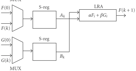
MUX
LRA
F(0)
F(k)
G(0)
G(k) MUX
S-reg
S-reg
Ak
Bk
αFi+βGi F
(k+ 1)
Figure 1: Arithmetic processor for the spreading calculation scheme.
F(0)
F(k)
G(0)
G(k)
Ak
Bk
αFi−βGi
αGi+βFi
F(k+ 1)
G(k+ 1)
Figure2: Arithmetic processor for the crossed paired evaluation.
4. PROCESSOR IMPLEMENTATION
As mentioned inSection 3, the two main computing issues lead to different architectural counterparts. The development of a new function evaluation upon the previous one in a spreading calculation scheme is carried out by the processor presented inFigure 1that requires functionGto be known. The second scheme deals with the crossed paired calculation of theF andG functions. The corresponding processor is shown inFigure 2.
The implementation proposed uses an LRA (acronym for look-up table (LUT), register, reduction structure, and adder). The LUT contains all partial productsαAk+βBk;Ak,
Table5: Arithmetic processor estimations of area cost and time delay for 16 bits and one-bit fragmented data.
Hardware devices Occupied area Time delay
Multiplexer 0.25· ×2×16τa=8τa 0, 5τt
Shift register 0.5×16τa=8τa 15×0, 5τt=7, 5τt
LRA
LUT 40τa/Kbit×16 bits×16 cell=10τa 3.5τt×16 accesses=56τt
Register 0.5×16·τa=8τa 1τt
Reduction structure 4 : 2 + adder 4τa+ 16τa=20τa 3 red.×3τt+ lg 16τt=13τt
Arithmetic processor (Figure 1) 70τa 78τt
Arithmetic processor (Figure 2) 108τa 78τt
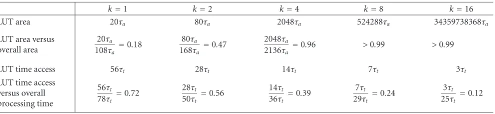
Table6: Relationship between area, time delay, and fragment lengthk, for 16 bits data for processor 2.
k=1 k=2 k=4 k=8 k=16
LUT area 20τa 80τa 2048τa 524288τa 34359738368τa
LUT area versus overall area
20τa 108τa =0.18
80τa 168τa =0.47
2048τa
2136τa =0.96 >0.99 >0.99
LUT time access 56τt 28τt 14τt 7τt 3τt
LUT time access versus overall processing time
56τt 78τt =0.72
28τt 50τt =0.56
14τt 36τt=0.39
7τt 29τt =0.24
3τt 25τt =0.12
On every cycle, the LUT is respectively accessed byAkandBk coming from the shift registers. Then, the partial products are taken out of the cells (partial products in the LUT are the hardware counterpart of the weighted primitives presented in Tables1and2). The overall partial productαFi+βGiis ob-tained by adding all the shifted partial products correspond-ing to all fragment inputsAk,Bk ofFi andGi, respectively. In the following iteration, both the new calculatedFi+1value and the nextGi+1 value are multiplexed and shifted before accessing the LUT in order to repeat the addressing process. The processor inFigure 2is different fromFigure 1in what concerns functionG. TheGvalues are obtained in the same way as forFbut the LUT forGis different from the LUT for
F.
4.1. Area costs and time delay estimation
In order to have the capability to make a comparison of com-puting resources, an estimation of the area cost and time delay of the proposed architectures is presented here. The model we use for the estimations is taken from the references [33,34]. The unitτa represents the area of a complex gate. The complex gate is defined as the pair (AND, XOR) that provides a meaningful unit, as these two gates implement the most basic computing device: the one bit full-adder. The unit
τtis the delay of this complex gate. This model is very use-ful because it provides a direct way to compare different ar-chitectures, without depending on their implementation fea-tures. As an example, the area cost and time delay for 16 bits one-bit fragmented data are estimated for both processors, as shown inTable 5.
If the fragments of the input data are greater than one bit, then the occupied area and the time delay access of the LUT vary. The relationship between area, time delay, and fragment lengthkfor 16 bits data is shown inTable 6for processor 2.
Table 6outlines that the LUT area increases exponentially withk, and represents an increasing portion of the overall area askincreases. The access time for the LUT decreases as 1/k. The percentage of access time versus overall processing time decreases slowly as 1/k. The trade-offbetween area and time has to be defined depending on the application.
The proposed architecture has also been tested in the XS4010XL-PC84 FPGA. Time delay estimation in usual time units can also be provided assumingτt≈1 ns.
4.2. Algorithmic stability
A complete study of the error is still under consideration and numerical results are not yet available except for particular cases [35]. Nevertheless, two main considerations are pre-sented: on one hand, the recursive calculation accumulates the absolute error caused by the successive round-offwhich is performed as the number of iterations increases, on the other hand, if round-offis not performed, the error can be-come lower as the length in bits of the result increases, but the occupied area as well as the time delay increase too. In what follows, both trends are analyzed.
Round-off is performed
accuracy of the mapping. A trade-offbetween the accuracy of the approximation (related to the number of calculated values) and the increasing calculation error must be found. Parallelization provides a mean to deal with this problem by defining more computing levels. TheNvalues of functionF that are to be calculated can be assigned to different com-puting levels (therefore different comcom-puting processors) in a tree-structured architecture, by spreadingNinto a product as follows:
N=N1·N2· · ·NP. (11)
– 1st computing level:F0is the seed value that initializes the calculation ofN1new values,
– 2nd computing level: theN1 obtained values are the seeds that initialize the calculation ofN1·N2new val-ues (N2values per eachN1).
And so on until achieving the
– pth computing level: the Np−1 obtained values are the seeds that complete the calculation of N = N1· N2· · ·Npnew values (Npvalues per eachNp−1). If the error for one value calculation is assumed to beε, the overall error afterNvalues calculation is
– for sequential calculation=Nε=N1·N2· · · · ·Npε, – for calculation by a tree structured architecture =
(N1+N2+· · ·+Np)ε.
The parallelized calculation decreases the overall error without having to decrease the number of points. The min-imum value for the overall error is obtained when the sum (N1+N2+· · ·+Np) is minimized, that is to say when allNi in the sum are relatively prime factors.
It can be mentioned that the time delay calculation fol-lows a similar evolution scheme as the error. ConsideringT as the time delay for one value calculation, the overall time delay is
– for sequential calculation=NT=N1·N2· · · · ·NpT, – for calculation by a tree structured architecture =
(N1+N2+· · ·+Np)T.
The minimization of the time delay is also obtained when theNiare relatively prime factors.
For the occupied area, the precise structure of the tree in what concerns the depth (number of computing levels) and the number of branches (number of calculated values per processor) is quite relevant for the result. The distribu-tion of theNiis crucial in the definition of some improving tendencies. The number of processorsPin the tree-structure can be bounded as follows:
P=1 +N1+N1·N2+N1·N2·N3
+· · ·+N1·N2·N3· · · · ·Np−1<1 + (p−1)N p .N
(12)
Pincreases at the same rate as the number of computing levels p, but the growth can be contained ifNpis the maxi-mum value of allNi, that is to say in the last computing level
p−1, the number of calculated values per processor is the highest. It can be observed that the parallel calculation in-volves much more processors than sequential one processor.
Summarizing the main ideas
(i) The parallel calculation provides benefits on error bound and time delay whereas sequential calculation performs better in what concerns area saving.
(ii) A trade-offmust be established between the time de-lay, the occupied area, and the approximation accuracy (through the definition of the computing levels).
Round-off is not performed
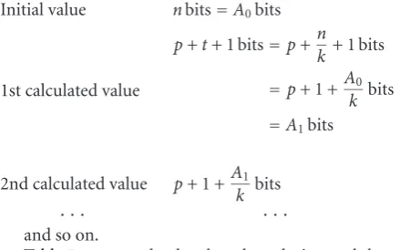
As explained in Section 2, we assume the first input data length is n, the data have been fragmented (n = kt), and the partial products in the cells are pbits long. Iftaccesses have been performed to the table andtpartial products have to be added, the first result will be p+t+ 1 bits long (tbits represent the increase caused by the corresponding shifts plus one bit for the last carry). The second value has to be calculated in the same way so that the p+t+ 1 bits of the feedback data isk-fragmented and the process goes on. This recursive algorithm can be formalized as follows:
Initial value nbits=A0bits
1st calculated value
p+t+ 1 bits=p+n
k+ 1 bits =p+ 1 +A0
k bits =A1bits
2nd calculated value p+ 1 +A1
k bits
· · · · · ·
and so on.
Table 7presents the data length evolution and the corre-sponding error forn= p=16, 32, and 64 bits data, as well as the number of calculated values that lead to the maximum data length achievement.
Table7: Data length evolution and error versus number of calculated values forn=p=16, 32, and 64 bits.
Initial data length (bits) Fragment length Final data length (bits) Length increase rate Number of calculated values Error
16
k=2 34 112% 9 2−34
k=4 23 44% 4 2−23
k=8 19 19% 2 2−19
k=16 18 12.5% 2 2−16
32
k=2 66 106% 10 2−66
k=4 44 37.5% 5 2−44
k=8 38 18.8% 4 2−38
k=16 35 9.4% 3 2−35
k=32 34 6.2% 2 2−34
64
k=2 130 103% 11 2−130
k=4 86 34.3% 6 2−86
k=8 74 15.6% 4 2−74
k=16 69 7.8% 4 2−69
k=32 67 4.7% 2 2−67
k=64 66 3.1% 2 2−66
5. GENERIC CALCULATION SCHEME FOR
INTEGRAL TRANSFORMS
In this section, a generic calculation scheme for integral transforms is presented. The DFT is taken as a paradigm and some other transforms are developed as applications of the DFT calculation.
5.1. The DFT as paradigm
Equation (13) is the expression of the one-dimensional dis-crete Fourier transform. Let us haveN=2M=2n,
F(u)= N1 N
−1
x=0
f(x)W2uxM, whereWN=exp−2jπ
N .
(13)
The Cooley and Tukey algorithm segregates the FT in even and odd fragments in order to perform the successive folding scheme, as shown in (14):
F(u)=1
2
Feven(u) +Fodd(u)W2uM
,
F(u+M)=1
2
Feven(u)−Fodd(u)W2uM
,
Feven(u)=M1 M−1
x=0
f(2x)WMux,
Fodd(u)= 1
M
M−1 x=0
f(2x+ 1)WMux.
(14)
For any u ∈ [0,M[, the Cooley and Tukey algorithm starts by setting theM initial two-point transforms. In the second step M/2 four-point transforms are carried out by combining the former transforms and so on till to reach the last step, where one M-point transform is finally obtained.
For values ofu∈[M,N[ no more extra calculations are re-quired as the corresponding transforms can be obtained by changing the sign, as shown by the second row in (14).
Our method enhances this process by adding a new seg-regation held by both real (R) and imaginary (I) parts in or-der to allow the crossed evaluation presented at the end of Section 3. Due to the fact that two segretations are consid-ered (even/odd, real/imaginary) there will be, for eachu, four transforms, which areRp,qeven,Rp,qodd,Ip,qeven, and Ip,qodd where p,q denote the step of the process and the number of the transform in the step, respectively,p∈[0,n−1], and
q∈[0, 2n−1−1].
Equations (15), (16), and (17) show the first, the sec-ond, and the last steps of our process, respectively, for any
u ∈ [0,M[. Parameters αp(u) = cospπu/M andβp(u) =
sinpπu/Mdefine the stepp. Theuargument has been omit-ted in (16) and (17) in order to clarify the expansion. In the first step, M two-point real and imaginary transforms are set in order to start the process. In the second stepM/2 real and imaginary transforms are carried out following the calculation scheme shown in (9). At the end of the process, one real and one imaginaryM-point transform are achieved and, without any more calculation, the result is deduced for
u∈[M,N[. As observed in (16) and (17), each step involves the results of Rand I obtained in the two previous steps; therefore, in each step the number of equations is halved. Af-ter the first step, a sum is added to the weighted primitive. This could have an effect on the LUT as the parameter set becomes (α,β, 1),
u∈[0,M[
R0,0 even(u)= f(0) +α0(u)f
2n−1,
R0,1 odd(u)= f
2n−2+α0(u)f
2n−2+ 2n−1,
· · ·
R0,M−1 odd(u)=f2 + 22+· · ·+ 2n−2 +α0(u)f
I0,0 even(u)= −β0(u)f
2n−1,
I0,1 odd(u)= −β0(u)f
2n−2+ 2n−1,
· · · I0,M−1 odd(u)= −β0(u)f
2 + 22+· · ·+ 2n−2+ 2n−1, (15)
R1,0 even=R0,0 even+α1R0,1 odd−β1I0,1 odd
=R0,0 even+R0,1 odd⊕I0,1 odd, I1,0 even=I0,0 even+β1R0,1 odd+α1I0,1 odd
=I0,0 even+R0,1 odd⊕I0,1 odd, R1,1 odd=R0,2 even+α1R0,3 odd−β1I0,3 odd
=R0,2 even+R0,3 odd⊕I0,3 odd, I1,1 odd=I0,2 even+β1R0,3 odd+α1I0,3 odd
=I0,2 even+R0,3 odd⊕I0,3 odd,
· · ·
R1,M/2−1 odd=R0,M/2 even+α1R0,M/2+1 odd−β1I0,M/2+1 odd
=R0,M/2 even+R0,M/2+1 odd⊕I0,M/2+1 odd, I1,M/2−1 odd=I0,M/2 even+β1R0,M/2+1 odd+α1I0,M/2+1 odd
=I0,M/2 even+R0,M/2+1 odd⊕I0,M/2+1 odd,
(16) R=Rn−1,0=Rn−2,0 even+αn−1Rn−2,1 odd
−βn−1In−2,1 odd
=Rn−2,0 even+Rn−2,1 odd⊕In−2,1 odd, I=In−1,0=In−2,0 even+βn−1Rn−2,1 odd
+αn−1In−2,1 odd
=In−2,0 even+Rn−2,1 odd⊕In−2,1 odd,
(17)
u∈[M,N[
R=Rn−1,0=Rn−2,0 even−αn−1Rn−2,1 odd +βn−1In−2,1 odd
=Rn−2,0 even−Rn−2,1 odd⊕In−2,1 odd, I=In−1,0=In−2,0 even−βn−1Rn−2,1 odd
−αn−1In−2,1 odd
=In−2,0 even−Rn−2,1 odd⊕In−2,1 odd.
(18)
The number of operations has been used as the main unit to measure the computational complexity of the proposal. The operation implemented by the weighted primitive has been denoted as weighted sum WS, and the simple sum as SS. The calculations take into account both real and imagi-nary parts for anyuvalue. The initial two-point transforms are assumed to be calculated. An inductive scheme is used to carry out the complexity estimations.
(i)N=4,n=2,M=2
F(0): 1 SS
F(1): 2×3=6 WS
F(2): deduced fromF(0), 1 SS
F(3): deduced fromF(1), 2×1=2 WS (change of sign) Overall: 8 WS and 2 SS.
(ii)N=8,n=3,M=4
F(0): 3 SS
F(1),F(2) andF(3) =14 WS
F(4): 3 SS
F(5),F(6) andF(7)=2×3 =6 WS (change of sign) Overall: 20 WS and 6 SS.
(iii)N=16,n=4,M=8
F(0): 7 SS
F(1),F(2),F(3),. . .,F(7) =30 WS
F(8): 7 SS
F(9),. . .,F(15)=2×7 =14 WS (change of sign) Overall: 44 WS and 14 SS.
From these results two induced calculation formulas can be proposed referring to the count of needed weighted sums and simple sums,
WS(n)=2×WS(n−1) + 4,
SS(n)=2×SS(n−1) + 2. (19)
Proof. Starting from WS(1) = 2 and SS(1) = 0, for anyn,
n >1, it may be assumed that
WS(n)=2(2n−1) + (2n−2)=2n+ 1 + 2n−4,
SS(n)=2n−2. (20)
By the application of the inductive scheme, after substi-tutingnbyn+ 1 the formulas become
WS(n+ 1)=2n+ 2 + 2n+ 1−4,
SS(n+ 1)=2n+ 1−2. (21)
Comparing the expressions fornandn+ 1, it can be no-ticed that
WS(n+ 1)=2×WS(n) + 4,
SS(n)=2×SS(n−1) + 2. (22)
The proposed formulas (see (19)) have been validated by this proof.
Comparing with the Cooley and Tukey algorithm, where
M(n) is the number of multiplications andS(n) the number of sums, we have
M(n+ 1)=2×M(n) + 2n,
S(n+ 1)=2×S(n) + 2n+1. (23) The contribution of the weighted primitive is clear as we compare (19) and (23). The quotientM(n)/WS(n) in-creases linearly versusn. The same occurs with the quotient
S(n)/SS(n) but with a steeper slope. So, the weighted primi-tive provides best results asngrows.
5.2. Other transforms
Hartley transform
LetH(u) be the discrete Hartley transform of a real function
f(x):
H(u)=N1 N
−1
x=0 f(x)
cos2πux
N + sin
2πux
N
,
where R(u)=N1 N
−1
x=0
f(x) cos2πux
N ,
I(u)= N1 N
−1
x=0
f(x) sin2πux
N .
(24)
H(u) is the transformed sequence that can split into two fragments:R(u) corresponds to the cosine part andI(u) to the sine part. The whole previous development for the DFT can be applied but the last stage has to perform an additional sum of the two calculated fragments,
H(u)=R(u) +I(u). (25) The number of simple sums increases as one last sum must be performed per eachuvalue. Nevertheless, (19) suits because only the initial value varies, SS(1)=2,
WS(n)=2×WS(n−1) + 4,
SS(n)=2×SS(n−1) + 2. (26)
Cosine/sine transforms
LetC(u) be the discrete cosine transform of a real function
f(x):
C(u)=e(k) N−1
x=0
f(x) cos(2x+ 1)πu
2N . (27)
C(u) is the transformed sequence that can split into two fragments as follows:
f(x) cos(2x+ 1)πu 2N
= f(x) cos
πux
N +2πuN
= f(x)
cosπux
N cos2πuN −sin
πux N sin2πuN
.
(28)
So that (27) leads to (29)
C(u)=e(k) N−1
x=0 f(x)
cosπux
N cos2πuN−sin
πux N sin2πuN
.
(29)
Then, cos[πu/2N] and−sin[πu/2N] are constant values for eachuvalue and can lay outside the summation:
C(u)=e(k)
αu N−1
x=0
f(x) cosπux
N +βu
N−1 x=0
f(x) sinπux
N
,
where cosπu
2N =αu,−sin
πu
2N =βu. (30)
Both fragments,R(u) (for the cosine part) andI(u) (for the sine part), can be carried out under the DFT calcula-tion scheme and combined in the last stage by an addicalcula-tional weighted sum:
C(u)=αuR(u) +βuI(u). (31)
A similar result could be inferred for sine transform with the following parameter values: cos(πu/2N) = αu, sin(πu/2N)=βu.
The number of weighted sums increases because of the last weighted sum that must be performed, see (31). The equation has been modified as the constant value in WS(n) varies. The reason is that the initial value WS(1)=3,
WS(n)=2×WS(n−1) + 3,
SS(n)=2×SS(n−1) + 2. (32)
Summarizing
The calculation based upon the DFT scheme leads to an easy approach for the calculation of the DHT and the DCT/DST, as expected. This scheme can be extended to other integral transforms with trigonometric kernel.
6. COMPARISON WITH OTHER PROPOSALS
AND DISCUSSION
In this section, some hardware implementations for the cal-culation of the DFT, DHT, and DCT are presented in order to provide a comparison for the different performances in terms of area cost, time delay, and stability.
6.1. DFT
Table8: Critical path of the basic calculation module in the BDA architecture.
Preprocessor P/S RAM Adder + Acc Post-processor 4-point DFT Overall
Time per column 13.71 ns 12.45 ns 14.06 ns 17.7 ns 10.35 ns 68.27 ns Critical path 17.7 ns 17.7 ns 17.7 ns 17.7 ns 17.7 ns 88.5 ns
Table9: Comparison between the hardware needed by BDA and our architecture implementations.
N Devices implementing the DBA architecture Devices implementing our proposal
16 5 buffers, 1 CORDIC processor, P/S-R, 1 rotator, 4 (4×16) bits RAMs, 16 MAC
4 MUX, 4 S-R, 2 (64×16) bits LUTs 4 registers, 4 red-structures 4 adders
64 5 buffers, 1 CORDIC processor, P/S-R, 1 rotator, 4 (16×16) bits RAMs, 16 MAC
512
9 buffers, 1 CORDIC processor, 2 P/S-R, 1 rotator, 8 (8×16) bits RAMs, 32 MAC 1 transposition memory
4096
9 buffers, 1 CORDIC processor, 2 P/S-R, 1 rotator, 8 (16×16) bits RAMs, 32 MAC 1 transposition memory
Table10: Comparison between the BDA and our architecture implementations in terms ofτaandτt.
N BDA architecture Our proposal
Area Time delay Area Time delay 1116 314τa 3.3 103τt
336τa
1.248 103τ t
1164 344τa 13.2 103τt 4.992 103τt
1512 632τa 105.6 103τt 39.936 103τt
4096 672τa 844.8 103τt 119.808 103τt
needed to reorder the partial products that are involved in the basic four points operation. The number of operations of this proposal isO((N1/4M)WL) whereN1is the length of the transform,M =4 in the design, andWLis the data length. When the transform is longer as 64 points,N1is substituted by theN1×N2.Table 8shows the results obtained by the syn-opsis implementation of the circuit that has been described in Verilog HDL.
In order to compare the performance of our architecture and that of the BDA, an estimation of the occupied area and time delay is provided. The devices for both implementa-tions are listed inTable 9and evaluated in terms ofτt and
τainTable 10. For the crossed evaluation scheme, the archi-tecture is double because of the two segregations (even/odd and real/imaginary); 64 cells LUTs are assumed as the param-eter set is (α,β, 1). Data is 16 bits long for any proposal. In Table 10, neither the rotator nor the CORDIC processor has been considered in the BDA implementation because the ref-erence does not facilitate any detail upon their structure. The estimations of the time delay are based on the author’s indi-cations and presented in terms ofτaandτtunits.
It can be observed that the BDA architecture is worse than the crossed one in what concerns the occupied area be-cause the BDA hardware needs to be increased stepwise when the number of points of the transforms increases. The time
delay is lower for the crossed architecture than for the BDA for the values ofNthat have been considered and will remain lower for anyN, because it achieves a linear growing in both implementations.
Table 11summarizes the hardware cost as well as the time delay of proposals for the Fourier transform calculation pre-sented by different authors [13,37–40]. The four proposals in the beginning of the list have based their design on sys-tolic matrices, the following one on adders and the others on distributed arithmetic (the DA is a generic distributed arith-metic approach). At the end of the list appears our proposal. Average computation time is indicated as
N
1 4
WLTROM+ 2TADD+TLATCH
. (33)
It appears that our proposal is the best in what concerns the hardware resources but time delay has a linear growth with respect toN(number of points of the transform) and with the data precision. It can be remembered that parallel architecture may present a better performance for this case.
6.2. DHT
Table11: Comparison between our proposal and other ones.
Memory Adders Multipliers Shift registers
P/S
registers CORDIC
Average calculation time
Chang and
Chen[37] 0 N N 6N 0 0
N×(2Tmult+ 2Tadd+Tlatch)
Fang and
Wu[38] 0 2N+ 6 N+ 4 6N 0 0
N×(2Tmult+ 2Tadd+Tlatch)
Murthy and
Swamy[39] 0 N N 10N 0 0
N×(2Tmult+ 2Tadd+Tlatch)
Chan and
Panchanathan[13] 0 N N 8N 0 0
N×(2Tmult+ 2Tadd+Tlatch)
Chang et al.
[40] 4N−4 (RAM) 6N+ 7 0 4N−2 0 0
N/2×(Tsum+
Tlatch+Tadd)
DA design N
4x2 (ROM)
N2
4 0 5N N 0
WL×(TROM+ 2Tadd+Tlatch)
BDA design N
4x2 (ROM)
N
4 + 4 0 3N
N
4
N
4 + 4
N×WL/4×(TROM+ 2Tadd+Tlatch)
Our proposal 2×WL×23(ROM) 2 + 2 0 2 0 0 (3(NN/−21)−W2)×WLTROM+ L×Tadd
Table12: Lowest known operation counts (real multiplications + additions) for power-of-two DHT and corresponding DFT algorithms versus our proposal (weighted sums + simple sums).
SizeN DHT (split-radix FHT) DFT (split-radix FFT) Our proposal
4 0 + 8=8 0 + 6=6 8 + 6=14
8 2 + 22=24 2 + 20=22 20 + 14=34
16 12 + 64=76 10 + 60=70 44 + 30=74
32 42 + 166=208 34 + 164=198 92 + 62=154
64 124 + 416=540 98 + 420=518 188 + 126=314
128 330 + 998=1328 258 + 1028=1286 380 + 254=634
256 828 + 2336=3164 642 + 2436=3078 764 + 510=1274
512 1994 + 5350=7344 1538 + 5636=7174 1532 + 1022=2554
1024 4668 + 12064=16732 3586 + 12804=16390 3068 + 2046=5114
operations) than the corresponding DFT algorithm special-ized for real inputs (or outputs), as proved by Sorensen et al. in 1987 [19]. To illustrate this, Table 12 lists the lowest known operation counts (real multiplications + additions) for the DHT and the DFT for power-of-two sizes, as achieved by the split-radix Cooley-Tukey FHT/FFT algorithm in both cases. Notice that, depending on DFT and DHT implemen-tation details, some of the multiplications can be traded for additions or vice versa. The third column of the table esti-mates the operation counts (weighted sums + simple sums) to be performed by our proposal, following (19).
As expected, our proposal behaves better in what con-cerns the operation counts than both the DHT algorithm and the corresponding DFT algorithm specialized for real inputs or outputs. With respect to the particular hardware imple-mentations, as the DFT has already been compared above with our proposal, the concluding remarks related to the DHT have to be deduced.
Table13: Normwise forward stability of DHT-I (N) for 16, 32, and 64 bits data.
N log2(N) u=2−16 u=2−32 u=2−64
16 4 13.292163u=23.742−16=2−19.74 13.292163u=23.742−32=2−35.74 13.292163u=23.742−64=2−67.74 32 5 17.722908u=24.162−16=2−20.16 17.722908u=24.162−32=2−36.16 17.722908u=24.162−64=2−68.16 64 6 22.153605u=24.482−16=2−20.48 22.153605u=24.482−32=2−36.48 22.153605u=24.482−64=2−68.48 128 7 24.752−16=2−20.75 24.752−32=2−36.75 24.752−64=2−68.75 256 8 24.972−16=2−20.97 24.972−32=2−36.97 24.972−64=2−68.97 512 9 25.162−16=2−21.16 25.162−32=2−37.16 25.162−64=2−69.16 1024 10 25.332−16=2−21.33 25.332−32=2−37.33 25.332−64=2−69.33 2048 11 25.492−16=2−21.49 25.492−32=2−37.49 25.492−64=2−69.49 4096 12 25.632−16=2−21.63 25.632−32=2−37.63 25.632−64=2−69.63 8192 13 25.752−16=2−21.75 25.752−32=2−37.75 25.752−64=2−69.75 16384 14 25.872−16=2−21.87 25.872−32=2−37.87 25.872−64=2−69.87
The computational complexity is calculated for all types DHT-X, X =I, II, III, and IV but for comparison with our results we will consider the best result which is for X=I.
The number of additions is denoted byα(DHT-I,N) and the number of multiplications byμ(DHT-I,N):
(DHT-I,N)= 3
2Nlog2(N)− 3 2N + 2,
μ(DHT-I,N)=Nlog2(N)−3N+ 4.
(34)
As seen in the paper, the operation error follows the IEEE precision arithmeticu=2−24oru=2−53depending on the precision of the mantissa (24 or 53 bits, resp.). The round-offalgorithmic errors are related to the structure of the in-volved matrices and for direct calculation the round-offerror is evaluated as a squared distance bounded by an expression
≈kNu. The numerical stability is measured bykN that can be understood as the relative error on the output vector (of the mapping previously defined). For any X, a different expres-sion for kN is obtained for the corresponding DHT-X(N). AllkN expressions are similar and have linear dependence of log2N. For example, the normwise forward stability for
DHT-I(N) is
4 3
√
3 +3 2
√
2log2N−1+O(u)
u.
(35)
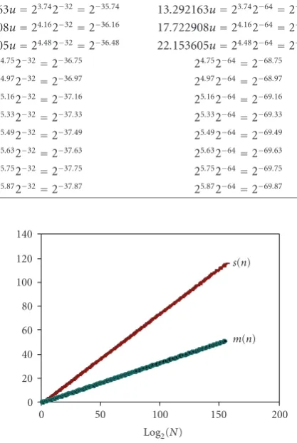
As far as we can compare this very deep and strong the-oretical approach with our method that is rather empirical, the results that can be taken into account are the computa-tional cost and the stability of the algorithms. To make easier the comparison with our paper in what concerns the num-ber of operations to be performed, a recursive formulation of (DHT-I,N) andμ(DHT-I,N)=forN=2nhas been de-duced from (34):
α(n)=2α(n−1) + 3.2n−2,
μ(n)=2μ(n−1) + 2n−4. (36)
0 20 40 60 80 100 120 140
0 50 100 150 200
Log2(N)
s(n)
m(n)
Figure3: Growing ratess(n) andm(n) versusn.
Table14: Number of multiplication and addition operations for different 4×4 DCTs.
Operation Fast algorithms Our proposal
[48] [49] [47]
Multiplication 512 256 172 45
Addition 496 480 963 14
The initial values are forn=1, following (34):
α(1)=3
2·2.1− 3
2·2 + 2=2,
μ(1)=2·1−3 + 4=3.
(37)
The comparison between (19) and (36) (WS(n) versus
μ(n) and SS(n) versusα(n)) outlines thatα(n) andμ(n) in-crease at a higher speed than WS(n) and SS(n), respectively,
(i) for alln,α(n)>SS(n), (ii) forn >6,μ(n)>WS(n).
Figure 3represents the growing ratess(n)=α(n)/SS(n) andm(n)=μ(n)/WS(n) versusn.
The value of the normwise forward stability in the case of DHT-I (N) is (((4/3)√3 + (3/2)√2)(log2N−1) +O(u))u=
Table15: Number of recursive cycles for differentN×NDCT recursive structures.
N×N Row-column method with transposition memory
Recursive
algorithm Our proposal
[42] [43] [45] [46] [47]
Power of two
8×8 1024 1024 800 256 220 189
16×16 8192 8192 5952 2048 1756 765
32×32 65526 65536 45696 16384 14044 3069
64×64 524288 524288 357632 131073 112348 12285
128×128 4194304 4194304 2828800 1948567 898780 49149
Number of recursive kernels 1 1 1 2 2 0
Size of transposition memory ON2 ON2 ON2 ON2 0 0
Table16: Comparison between the hardware needed by the recursive architecture versus that of the implementation of our proposal for 4×4 DCT transform.
N×N Devices implementing the recursive architecture Devices implementing our proposal
4×4
1×Data memory buffer,
4×MUX, 4 S-R, 2×(64×16) bits LUTs 4×registers,
4×reduction structures 4×adders
2×adders 2×1–4 DEMUX 1×CMP
1×Condensed counter
(2×ripple connected mod-4 counters) 1×Condensed index generator (2 S-R, 2 shifters, 3 adders) 2×Recursive input buffer 2×1D DCT/DST IIR
ofTable 7, the previous formula has been calculated for the casesu = 2−16, 2−32, and 2−64bits and for different values ofN.
The comparison between Tables7and13shows that for 16 bits (fragmentation lengthsk =2 andk=4), for 32 bits data (k =2, 4, and 8) and for 64 bits data (k=2, 4, and 8) our algorithm behaves better.
6.3. DCT
The search for recursive algorithms with regular structure and less computation time remains an active research area. The recursive algorithms for computing 1D DCT are highly regular and modular [41–47]. However, a great number of cycles are required to compute the 2D transformation by us-ing 1D recursive structures. For computus-ing the 2D DCT by row-column approaches, the row (column) transforms of the input 2D data are first determined. A transposition mem-ory is required to store those temporal results. Finally, the 2D DCT results are obtained by the column (row) trans-forms of the transposed data. The RAM is usually adopted as the transposition memory. This approach has disadvantages such as higher-power consumption and long access time. Chen et al. develop in 2004 a new recursive structure with fast and regular recursion to achieve fewer recursive cycles with-out using any transposition memory structure [48]. The 2D recursive DCT/IDCT algorithms are developed considering
that the data with the same transform base can be pre-added such that the recursive cycles can be reduced. First, the 2D DCT/IDCT is decomposed into four portions which can be carried out either by 1D DCT or 1D DST (discrete sine trans-form). Based on the use of Chebyshev polynomials, efficient transform kernels are obtained for the 1D DCT and the DST. A reduction on the number or recursive cycles is achieved by a further folding on the inputs of the transform kernels. Con-sidering other fast algorithms, theN×NDCT which maps the 2D index of the input sequence into the new 1D index is decomposed intoNlength-N1D DCTs [49,50].Table 14 presents the number of multiplication and addition opera-tions for these fast algorithms, for the case of 4×4 DCTs. Our proposal can be compared by assimilating the weighted sums and the multiplications (see (32)).
So, the overall time delay for the 2D may be the same as for the 1D and the comparison with our proposal can be done as we assimilate the number of recursive cycles with the number of weighted sums to be performed following (32).
It can be outlined that our proposal has a better perfor-mance than the other ones, namely fast and recursive algo-rithms, in what concerns the number of recursive cycles. In [48] the chip area can be estimated as we depict the hardware recursive circuitry. Table 16 summarizes the hardware de-vices of the recursive architecture compared with our pro-posal for 4×4 DCT transform.
It can be observed that the devices for the implementa-tion of the recursive architecture are numerous. Therefore, greater values forN×Nmay imply an increase of the chip area; the reason is the growth of the storing memory required for the buffers and for the number of outputs of the demul-tiplexer. Reference [48] does not offer any estimation of the time delay of the calculation. Our proposal implementation is very simple and has no variation related to the amount of devices when the number of calculated values varies. With respect to the time delay of the calculation in [48], as far as we can suppose, it can be estimated by analyzing the critical path of the depicted circuit. It seems to be higher than our proposal’s one.
7. CONCLUSIONS
This paper has presented an approach to the scalability prob-lem caused by the exploding requirements of computing re-sources in function calculation methods. The fundamentals of our proposal claim that the use of a more complete prim-itive, namely a weighted sum, converts the calculation of the function values into a recursive operation defined by a two-input table. The strength of the method is concerned with the fact that the operation to be performed is the same for the evaluation of different functions (elementary or not). There-fore, only the table must be changed because it holds the fea-tures of the concrete evaluated function in the parameter val-ues. This method provides a linear computational cost when some conditions are fulfilled. Image processing transforms that involve combined trigonometric functions provide an interesting application field. A generic calculation scheme has been developed for the DFT as paradigm. Other image transforms namely the DHT and the DCT/DST are analyzed under the scope of the DFT. When comparing with other well-known proposals, it has been confirmed that our ap-proach provides a good trade-offbetween hardware resource and time delay saving as well as encouraging partial results in what concerns error contention.
REFERENCES
[1] R. Chamberlain, E. Lord, and D. J. Shand, “Real-time 2D floating-point fast Fourier transforms for seeker simulation,” inTechnologies for Synthetic Environments: Hardware-in-the-Loop Testing VII, R. L. Murrer Jr., Ed., vol. 4717 ofProceedings of SPIE, pp. 15–23, Orlando, Fla, USA, July 2002.
[2] P. Yan, Y. L. Mo, and H. Liu, “Image restoration based on the discrete fraction Fourier transform,” inImage Matching and
Analysis, B. Bhanu, J. Shen, and T. Zhang, Eds., vol. 4552 of Proceedings of SPIE, pp. 280–285, Wuhan, China, September 2001.
[3] W. A. Rabadi, H. R. Myler, and A. R. Weeks, “Iterative mul-tiresolution algorithm for image reconstruction from the mag-nitude of its Fourier transform,”Optical Engineering, vol. 35, no. 4, pp. 1015–1024, 1996.
[4] C.-H. Chang, C.-L. Wang, and Y.-T. Chang, “Efficient VLSI architectures for fast computation of the discrete Fourier transform and its inverse,”IEEE Transactions on Signal Pro-cessing, vol. 48, no. 11, pp. 3206–3216, 2000.
[5] S.-F. Hsiao and W.-R. Shiue, “Design of low-cost and high-throughput linear arrays for DFT computations: algorithms, architectures, and implementations,” IEEE Transactions on Circuits and Systems II, vol. 47, no. 11, pp. 1188–1203, 2000. [6] J. W. Cooley and J. W. Tukey, “An algorithm for the machine
calculation of complex Fourier series,”Mathematics of Com-putation, vol. 19, no. 90, pp. 297–301, 1965.
[7] P. N. Swarztrauber, “Multiprocessor FFTs,”Parallel Comput-ing, vol. 5, no. 1-2, pp. 197–210, 1987.
[8] C. Temperton, “Self-sorting in-place fast Fourier transforms,” SIAM Journal on Scientific and Statistical Computing, vol. 12, no. 4, pp. 808–823, 1991.
[9] M. C. Pease, “An adaptation of the fast Fourier transform for parallel processing,”Journal of the ACM, vol. 15, no. 2, pp. 252–264, 1968.
[10] L. L. Hope, “A fast Gaussian method for Fourier transform evaluation,”Proceedings of the IEEE, vol. 63, no. 9, pp. 1353– 1354, 1975.
[11] C.-L. Wang and C.-H. Chang, “A DHT-based FFT/IFFT pro-cessor for VDSL transceivers,” inProceedings of IEEE Interna-tional Conference on Acoustics, Speech, and Signal Processing (ICASSP ’01), vol. 2, pp. 1213–1216, Salt Lake, Utah, USA, May 2001.
[12] W.-H. Fang and M.-L. Wu, “An efficient unified systolic archi-tecture for the computation of discrete trigonometric trans-forms,” inProceedings of IEEE International Symposium on Cir-cuits and Systems (ISCAS ’97), vol. 3, pp. 2092–2095, Hong Kong, June 1997.
[13] E. Chan and S. Panchanathan, “A VLSI architecture for DFT,” inProceedings of the 36th Midwest Symposium on Circuits and Systems, vol. 1, pp. 292–295, Detroit, Mich, USA, August 1993. [14] R. V. L. Hartley, “A more symmetrical Fourier analysis applied to transmission problems,” Proceedings of the IRE, vol. 30, no. 3, pp. 144–150, 1942.
[15] R. N. Bracewell, “Discrete Hartley transform,”Journal of the Optical Society of America, vol. 73, no. 12, pp. 1832–1835, 1983.
[16] R. N. Bracewell, “The fast Hartley transform,”Proceedings of the IEEE, vol. 72, no. 8, pp. 1010–1018, 1984.
[17] R. N. Bracewell, The Hartley Transform, Oxford University Press, New York, NY, USA, 1986.
[18] R. N. Bracewell, “Computing with the Hartley transform,” Computers in Physics, vol. 9, no. 4, pp. 373–379, 1995. [19] H. V. Sorensen, D. L. Jones, M. T. Heideman, and C. S. Burrus,
“Real-valued fast Fourier transfer algorithms,”IEEE Transac-tions on Acoustics, Speech, and Signal Processing, vol. 35, no. 6, pp. 849–863, 1987.