Volume 2008, Article ID 647502,9pages doi:10.1155/2008/647502
Research Article
A Two-Microphone Noise Reduction System for
Cochlear Implant Users with Nearby Microphones—Part I:
Signal Processing Algorithm Design and Development
Martin Kompis,1Matthias Bertram,1, 2Jacques Franc¸ois,3and Marco Pelizzone4
1Department of ENT, Head and Neck Surgery Inselspital, University of Berne, CH-3010 Berne, Switzerland 2Bernafon Inc., Berne, CH-3018 Berne, Switzerland
3Laboratoire des Microprocesseurs, Ecole d’Ing´enieurs de Gen`eve, 1202 Geneva, Switzerland 4Clinique O.R.L., Hˆopital Universitaire de Gen`eve, 1211 Geneva, Switzerland
Correspondence should be addressed to Martin Kompis,[email protected]
Received 27 November 2007; Accepted 20 March 2008
Recommended by Chein-I Chang
Users of cochlear implant systems, that is, of auditory aids which stimulate the auditory nerve at the cochlea electrically, often complain about poor speech understanding in noisy environments. Despite the proven advantages of multimicrophone directional noise reduction systems for conventional hearing aids, only one major manufacturer has so far implemented such a system in a product, presumably because of the added power consumption and size. We present a physically small (intermicrophone distance 7 mm) and computationally inexpensive adaptive noise reduction system suitable for behind-the-ear cochlear implant speech processors. Supporting algorithms, which allow the adjustment of the opening angle and the maximum noise suppression, are proposed and evaluated. A portable real-time device for test in real acoustic environments is presented.
Copyright © 2008 Martin Kompis et al. This is an open access article distributed under the Creative Commons Attribution License, which permits unrestricted use, distribution, and reproduction in any medium, provided the original work is properly cited.
1. INTRODUCTION
Cochlear implant systems, that is, devices which stimulate the auditory nerve directly electrically in the cochlea, have become a successful method of treatment for bilaterally profoundly deaf patients. While speech understanding in quiet environments varies between patients but is often sat-isfactory for everyday use, insufficient speech understanding in noise is a major difficulty encountered by many users of cochlear implant systems [1,2].
Bilateral cochlear implantation is one method known to improve speech understanding in noise [1,3]. However, because of the relatively high cost involved and the need of a second implantation, for numerous users this is not currently an option.
A different approach to alleviate this problem is the use of directional multimicrophone noise reduction systems [4– 11]. Surprisingly, of the 3 major manufacturers of cochlear implant systems, today only one provides a system with multimicrophone noise reduction [7], and two do not [12, 13]. The system available on the market is relatively complex
and large (distance between microphone ports 19 mm) [7]. As the size of the speech processor is perceived by the users [14], we believe that a part of the reluctance of the manufacturers of cochlear implants to implement directional multimicrophone noise reduction systems in their products are concerns regarding additional size, complexity, and power consumption.
The aim of this investigation is to show one possibility to build efficient, physically small, flexible, and computationally inexpensive two-microphone noise reduction systems. It is our aim to show that such systems are realistic and provide a substantial benefit for cochlear implant users and hope to speed broader availability of such systems in commercially available cochlear implant systems.
Front microphone
Delay D3
− − +
(a) (b) (c) Output (e)
Delay D1 Delay
D2
Adaptive filterW
−
Target signal detection
Leakage control
(a) (b) (y)
(a) and (a) or (b) and (b) Rear
microphone
(a) (e)
(d)
Figure1: Block diagram of the two-microphone noise reduction system with nearby microphones.
This paper is organized as follows. In Section 2, the basic beamforming algorithm is described. In Section 3, two supporting algorithms are presented and evaluated. In Section 4, a portable prototype system is presented.
2. BASIC BEAMFORMING ALGORITHM
Figure 1shows a schematic drawing of the basic beamform-ing algorithm. It is similar to several algorithms proposed earlier [4,8,16,17]. One difference between these algorithms is the use of an adaptive finite impulse filter with several (N > 1) filter coefficients instead of an adjustable gain [16,17], corresponding to a filter withN = 1 coefficient. Another difference is the use of an end-fire microphone array rather than broadside array, that is, microphone ports which are in line with the target signal rather than one at each ear of the listener [4,8]. This microphone arrangement has been chosen to allow the system to fit into a single behind-the-ear housing. For the same reason, the device presented uses a very short intermicrophone distance (7 mm), which, however, is only a gradual difference.
The device works as follows (Figure 1). Using the two microphone output signals (a) and (a), two simple fixed directional units are formed, which are similar to conven-tional direcconven-tional microphones. One points to the front (signal (b) in Figure 1), and one to the back of the listener (b). Assuming that the target sound source lies in front of the listener, signal (b) will already contain predominantly target signal, signal (b) predominantly noise. The adaptive finite impulse response filter W withN coefficients w0 to
wN−1then further reduces the remaining noise in signal (b)
to form the output signal (c). This is achieved by first filtering (b) to generate an estimate (y) of the remaining noise in the delayed version of (b), and then subtracting it to from the noise reduced output signal (c). The filtering operation can be described as
y(k)=
N−1
n=0
b(k−n)·wn, (1)
wherekis the time index. A normalized LMS-algorithm [18, 19] is used to update the filter coefficients as follows:
wi(k+ 1)=wi(k) + 2μ·c(k)·b(k−i), (2)
whereμis the adaptation step size, normalized to
μ=α/2·N·b2, (3)
whereb2denotes average of the squared values of the signal
bover time segments corresponding to the filter length, and α is a dimensionless adaptation constant. The adaptation algorithm remains stable forαbetween 0 and approximately 2 [18,19]. Throughout this paper, an adaptation constant of α = 0.2 is used, resulting in reasonably short adapta-tion times (e.g., 2.4 milliseconds for the prototype device presented in Section 4) and a satisfactory convergence [9]. For adaptive beamformers using a broadside microphone placement, it has been shown that convergence is not a limiting factor to system performance and the normalized LMS-adaptation algorithm is sufficient [9]. Delay D3 is typically half of the length of the adaptive filter and used to optimize the amount of noise reduction [8,9].
3. SUPPORTING ALGORITHM
Two supporting algorithms, target signal detection and leakage control, are depicted in the lower part ofFigure 1. While leakage control is strictly an optional feature, a robust target signal detection scheme is essential for a satisfactory performance of the device in real acoustic environments.
3.1. Target signal detection
Signal (b) Square
x2 SmoothIIR S Detection parameter
d= S
S+N N
Stop adaptation ifd > T1
Signal (b) Square x2
Smooth IIR
Signal (a)
Signal (a)
Optional delaydS
Optional delaydN
Cross-correlation
for lags (−1, 0, 1)
S (value for lag= −1)
Maximum for lags
(0, 1) N
Detection parameter d= S
S+N Stop adaptation ifd > T2
Figure2: Two target signal detection schemes: top: delta-delta-algorithm. Bottom: multicorrelation algorithm.
will then be partly suppressed, leading to audible distortions of the output signals. This problem can be alleviated by detecting high SNRs and stopping filter adaptation during such time intervals. Even in fluent speech, there are still enough pauses and consequently enough time for the filter to adapt to the noise [20].
Several target-signal detection schemes have already been proposed [4,10,20–23] and used in adaptive beamformers with broadside microphone configurations [4, 20, 24]. As these algorithms are either computationally relatively expensive or not directly applicable in the proposed device with end-fire microphone configuration, we have developed and investigated two simple algorithms, the delta-delta-algorithm and the multicorrelation delta-delta-algorithm. Schematic diagrams of these two algorithms are shown inFigure 2.
The upper part of Figure 2 shows the delta-delta-algorithm. The signals (b) and (b) from the fixed directional units pointing to the front and to the back, respectively, are simply squared, smoothed, and compared. This is similar to the delta-sigma method used for broadside beamformers [20].
The performance of the delta-delta target signal detection algorithm was evaluated in two different simulated acoustic environments. The acoustic room simulation procedure used [25] calculates simulated impulse responses between acoustic sources and microphones in shoebox-shaped rooms, taking the head-shadow of the listener into account where the head is modeled as a rigid sphere with a diameter of 18.6 cm [9,25]. Two simulated acoustic environments were generated and used in this evaluation: one anechoic environment and one reverberant room with a reverberation time (time for the reverberant signal to decay by 60 dB) of 0.4 seconds and a volume of 34 m3. These values were chosen, as they represent
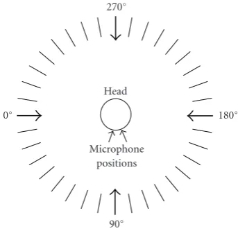
average values for small rooms in our own environment [9]. In each of the two simulated room, 36 omnidirectional sound sources were placed at the same height as the head of the listener, in a distance of 1 m from its center and at angles between 0◦and 350◦in steps of 10◦. This setting is depicted schematically inFigure 3. Two simulated impulse responses were calculated for each sound source and for each simulated room: one between the source and the front microphone,
Microphone positions
Head
0◦ 180◦
270◦
90◦
Figure 3: Placement of the 36 omnidirectional sound sources (at the outer end of each of the 32 lines and of the 4 arrows marked 0◦to 270◦) and of the two microphones (on the surface of the head, intermicrophone distance 7 mm) in the simulated acoustic environments used to evaluate the target signal detection algorithms.
and one between the source and the rear microphone, as indicated inFigure 3.
Two different signals, 5 seconds of white noise and 10 seconds of continuous speech, respectively, were filtered with the generated impulse responses and processed by the proposed delta-delta target signal detection algorithm. A sampling rate of 30, 000 s−1 was used to allow a simple
generation of delays in multiples of 33 microseconds in for the second target signal algorithm presented later in this section. The signals were low pass filtered at 4.6 kHz and downsampled to 10, 000 s−1. The filters labeled “smooth”
inFigure 5had exponential impulse responses with a time constant of 6.6 milliseconds.
Anechoic room White noise
90
10
0 0.2 0.4 0.6 0.8 1
Det
ection
p
ar
amet
er
d
0 50 100 150 200 250 300 350
Azimuth (◦) (a)
Reverberant room White noise
90 70 50 30 10
0 0.2 0.4 0.6 0.8 1
Det
ection
p
ar
amet
er
d
0 50 100 150 200 250 300 350
Azimuth (◦) (b) Anechoic room
Speech signal
90
10
0 0.2 0.4 0.6 0.8 1
Det
ection
p
ar
amet
er
d
0 50 100 150 200 250 300 350
Azimuth (◦) (c)
Reverberant room Speech signal
90
70
50
30
10
0 0.2 0.4 0.6 0.8 1
Det
ection
p
ar
amet
er
d
0 50 100 150 200 250 300 350
Azimuth (◦) (d)
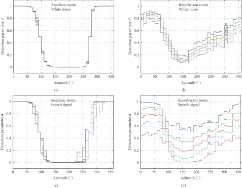
Figure4: Performance of the delta-delta target signal detection algorithm in simulated anechoic and reverberant environments as a function of the direction of incidence of the signal using either white noise or a speech signal. Percentiles denote the percentage of time, during which the detection parameterdwas lower than value indicated.
in percentiles of the time that the detection parameterdwas below a given value. It can be seen that this simple algorithm works considerably better in the anechoic environment than in the reverberant room and somewhat better for white noise than for the speech signal. Still, by choosing a reasonable thresholdT1, the algorithm can discriminate between high
and low SNR segments correctly for most of the time. The multicorrelation algorithm in the lower part of Figure 5is computationally more expensive. After optional delays (which can be ignored for the moment), three short-time cross-correlations between the two microphone signals (a) and (a) are calculated, using lags of−33 microseconds, 0 microsecond, and +33 microseconds and exponential filters with a time constant of 6.6 milliseconds. The value of the cross-correlation for the smallest lag is then compared to the maximum of the other two values.
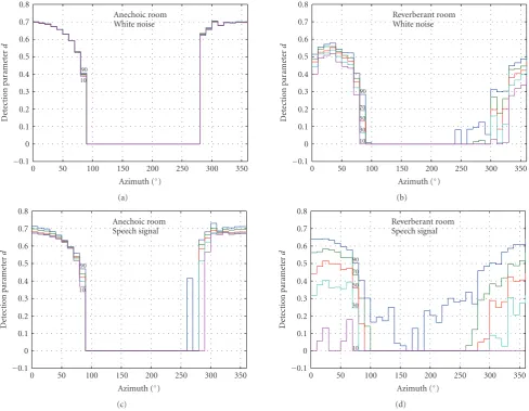
Figure 5shows results of the simulation using the multi-correlation algorithm. The experimental procedure was the same as described above for the delta-delta-algorithm. The delays, which are needed to calculate the cross-correlations,
were created by choosing different samples when downsam-pling the low-pass-filtered simulated signals from 30, 000 s−1
to 10, 000 s−1. It can be seen that the differentiation between
high and low SNRs is more reliable, that is, the percentiles are closer together, under reverberant conditions and between 100◦and 250◦.
Although slightly more complex, the multicorrelation algorithm gives rise to a new feature: it enables the design of adaptive beamformers with different or even adjustable opening angles. By choosing the angle, in which filter adaptation is stopped, we effectively chose the opening angle of the device, for example, the angle, in which sound sources are treated as target signal sources rather than noise to be cancelled. By introducing either an optional delaydSin the
signal path of the front microphone or a delaydN after the
Anechoic room White noise
90 10
−0.1 0 0.1 0.2 0.3 0.4 0.5 0.6 0.7 0.8
Det
ection
p
ar
amet
er
d
0 50 100 150 200 250 300 350
Azimuth (◦) (a)
Reverberant room White noise
90
70 50
30 10
−0.1 0 0.1 0.2 0.3 0.4 0.5 0.6 0.7 0.8
Det
ection
p
ar
amet
er
d
0 50 100 150 200 250 300 350
Azimuth (◦) (b) Anechoic room
Speech signal
90
10
−0.1 0 0.1 0.2 0.3 0.4 0.5 0.6 0.7 0.8
Det
ection
p
ar
amet
er
d
0 50 100 150 200 250 300 350
Azimuth (◦) (c)
Reverberant room Speech signal
90
70
50
30
10
−0.1 0 0.1 0.2 0.3 0.4 0.5 0.6 0.7 0.8
Det
ection
p
ar
amet
er
d
0 50 100 150 200 250 300 350
Azimuth (◦) (d)
Figure5: Performance of the multicorrelation target signal detection algorithm in simulated anechoic and reverberant environments as a function of the direction of incidence of the signal using either a white noise source or a speech signal. Percentiles denote the percentage of time, during which the detection parameterdwas lower than value indicated.
−60◦, where−60◦ corresponds to an azimuth of 300◦), the bottom left panel shows an opening angle of approximately 260◦between 100◦and−160◦(azimuth=200◦).
Figure 7 finally illustrates the effect of a target-signal detection/adaptation inhibition scheme on the entire beam-forming algorithm. In a simulated reverberant room and with a long adaptive filter (50 milliseconds), there is a clearly visible “beam,” tending slightly towards the side of the head with the microphones (90◦, seeFigure 3). The width of the “beam” varies in this case with the threshold parameter T1 of the delta-delta algorithm. Using a low value for T1,
signals with lower SNR are categorized as target signals, resulting in a wide beam (e.g.,T1 =0.1, left hand panel of
Figure 9). If higher values are chosen (e.g.,T1 = 0.4, right
hand panel ofFigure 9) only signal with relatively high SNR are considered to be target signals and the beam becomes narrow.
In this way, the target-signal detection/adaptation inhi-bition algorithm defines the opening angle of the entire beamforming system. If the signal source lies at an azimuth,
at which filter adaptation is not inhibited, for example, at the rear of the listener, the adaptation algorithm in (2) will reduce the variance of this signal at the output (c) or (e) of the beamformer. If, however, the signal source lies within the opening angle of the target signal detection, for example, in the front of the listener, adaptation in (2) will be inhibited (μ=0 in (2)) and the signal, now considered to be a target signal, will not be cancelled. Instead, it will be passed through delayD3 inFigure 1and, simultaneously, through filterW, which is adapted in the presence of signals considered to be noise, and the output (y) of which does, therefore, not match the target signal in the delayed version of (b), preventing its cancellation.
3.2. Leakage
Anechoic room Wide beam
90
10
0 0.2 0.4 0.6 0.8 1
Det
ection
p
ar
amet
er
d
0 50 100 150 200 250 300 350
Azimuth (◦) (a)
Anechoic room Narrow beam
90
10
−0.1 0 0.1 0.2 0.3 0.4 0.5
Det
ection
p
ar
amet
er
d
0 50 100 150 200 250 300 350
Azimuth (◦) (b) Reverberant room
Wide beam
90
10
−0.1 0 0.1 0.2 0.3 0.4 0.5
Det
ection
p
ar
amet
er
d
0 50 100 150 200 250 300 350
Azimuth (◦) (c)
Reverberant room Narrow beam
90
10
−0.1 0 0.1 0.2 0.3 0.4 0.5
Det
ection
p
ar
amet
er
d
0 50 100 150 200 250 300 350
Azimuth (◦) (d)
Figure6: Wide beam (left hand panels) and narrow beam (right hand panels) system obtained with the multicorrelation algorithm with optional delaysdSordN(see alsoFigure 5), respectively.
2 4
6 8
10 dB
180◦ 150◦
120◦
90◦
60◦
30◦
0◦
330◦
300◦ 270◦
240◦ 210◦
(a)
2 4
6 8
10 dB
180◦ 150◦
120◦
90◦
60◦
30◦
0◦
330◦
300◦ 270◦
240◦ 210◦
(b)
these directions, such as approaching cars, are not perceived sufficiently loud.
We believe that this is a minor problem. Beamforming can be switched offin these situations, adaptation takes a few milliseconds in which the signal is still well audible and— except under anechoic conditions—signal suppression is rarely great enough to actually miss a signal completely [15]. However, as situations outside of buildings may approach an anechoic environment, we propose a leakage control algorithm to alleviate this problem.
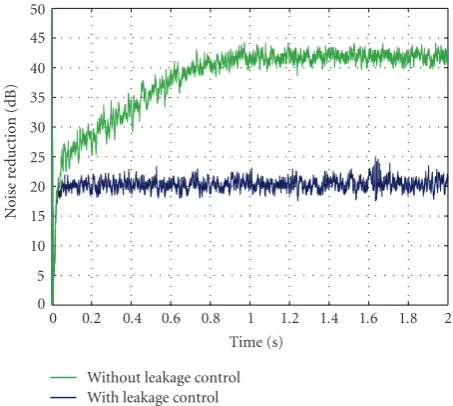
Figure 1 shows leakage control together with the pro-posed beamforming algorithm. The leakage control algo-rithm itself is very simple. The input and output signals of the device are squared, smoothed and compared. If the detected attenuation is greater than a preset value, for example, 20 dB, a portion of the microphone signal is delayed byD3 and “leaked” directly to the output (e). To minimize any unwanted comb-filter effect in the frequency domain by two slightly time-shifted versions of the same signal, signal (a) is delayed by the value ofD3 before being added to signal (c).
Figure 8shows the effect of the leakage control algorithm in a simulated situation using a white noise source in an anechoic environment. While noise suppression exceeds 40 dB after 1 second without leakage control, in this example it is limited to 20 dB when the algorithm is active.
3.3. Flexibility added by the supporting algorithms
With the above supporting algorithms, very simple or more complex beamformers can be designed, as needed. In accordance with the aims of this research stated in the introduction, we will concentrate on a small computationally inexpensive version inSection 4and [15].
Nevertheless, it is worth looking into the flexibility added by the supporting algorithms. If both, target-signal detection/adaptation inhibition and leakage control are implemented, a beamformer with two nearby microphones can be built, which is very flexible, as shown schematically in Figure 9. The opening angle (Figure 9(a)) and the maximum desired amount of noise reduction (Figure 9(b)) can be adjusted independently, either in an experiment, by the user or by an automated analysis of the current acoustical situation.
4. REAL-TIME REALIZATION OF AN EXPERIMENTAL BEAMFORMER
A portable beamforming device implementing the algorithm in Figure 1 was built in order to be able to perform experiments in real-time, with cochlear implant users and in real environments [15]. The system is built around a 16 bit fixed point digital signal processor (Motorola DSP56F826) and uses a Cirrus Logic CS42L50 sigma-delta Stereo CODEC with 24-bit quantization. Sampling rate was set at 16.8 kHz. The signal processing part is contained in a small housing (10.5×6.1×2.1 cm;Figure 10) which also holds the batteries, an LCD display and 4 control buttons. The output can directly drive the audio input of commercially available speech processors of cochlear implant
0 5 10 15 20 25 30 35 40 45 50
No
is
e
re
d
u
ct
io
n
(d
B
)
0 0.2 0.4 0.6 0.8 1 1.2 1.4 1.6 1.8 2 Time (s)
Without leakage control With leakage control
Figure8: Effect of leakage control in a simulated anechoic environ-ment. The maximum noise reduction is limited to approximately 20 dB.
(a) (b)
180◦ 0◦
90◦
270◦
Figure9: Schematic drawing of the possibilities to adjust the prop-erties of a directional noise reduction system using the proposed supporting algorithms: (a) beam width control using target signal detection algorithms and (b) maximum noise reduction using leakage control. The solid line represents an average setting and the dotted lines the range of adjustments, the radial axis denotes signal suppression arbitrary units.
systems. Two microphones are mounted in a behind-the-ear hbehind-the-earing aid housing, maintaining a distance of 7 mm between the microphone ports.
The fixed delay-and-subtract directional units were formed by using delaysD1,D2=59.5μs. The adaptive filter was 16 coefficients in length (952 microseconds), and the delayD3 was set to 1/2 of the length of the adaptive filter, that is, approximately 476 microseconds. A normalized LMS-algorithm was used, the adaptation held at 10% of the value, for which instability can be expected, leading to a theoretical adaptation time constant of 2.4 milliseconds. As a target signal detection, a delta-delta algorithm was implemented (time constant approximately 5 ms, detection thresholdT1=
0.2. The leakage control feature was not implemented. The device can be used in any one of 4 different modes. In mode (i), the output of the experimental device is the output signal (e) of the adaptive beamformer using the algorithm and parameters above; in mode (ii) the signal of one of the omnidrectional microphones (Figure 1signal (a)) is routed directly to the output; in mode (iii), the output signal of the directional fixed unit pointing to the front (Figure 1, signal (b)) is routed the output signal; and in mode (iv), the coefficients of the adaptive filter are frozen until mode (i) is restored.
5. SUMMARY
A two-microphone directional noise reduction system for cochlear implant systems was presented. Using the proposed supporting algorithms, target signal detection/adaptation inhibition and leakage control, simple or more sophisticated versions of the system can be built. Using the presented multicorrelation algorithm and leakage control, a very flexible device can be obtained, in which the opening angle of the beam and the maximum noise reduction can be defined separately. A portable prototype device using two nearby microphones spaced just 7 mm apart in a single behind-the-ear hbehind-the-earing aid housing was built. This device is used for further evaluations with cochlear implant users and in real acoustic environments [15].
ACKNOWLEDGMENT
This work was supported by the Swiss National Science Foundation, Grant no. 3238-056325/2.
REFERENCES
[1] J. M¨uller, F. Sch¨on, and J. Helms, “Speech understanding in quiet and noise in bilateral users of the MED-EL COMBI 40/40+ cochlear implant system,”Ear and Hearing, vol. 23, no. 3, pp. 198–206, 2002.
[2] M. Kompis, M. Bettler, M. Vischer, P. Senn, and R. H¨ausler, “Bilateral cochlear implantation and directional multi-microphone systems,” in Cochlear Implants, R. Miyamoto, Ed., International Congress Series, pp. 447–450, Elsevier, Amsterdam, The Netherlands, 2004.
[3] P. Senn, M. Kompis, M. Vischer, and R. H¨ausler, “Minimum audible angle, just noticeable interaural differences and speech intelligibility with bilateral cochlear implants using clinical
speech processors,”Audiology & Neurotology, vol. 10, no. 6, pp. 342–352, 2005.
[4] R. J. M. van Hoesel and G. M. Clark, “Evaluation of a portable two-microphone adaptive beamforming speech processor with cochlear implant patients,” Journal of the Acoustical Society of America, vol. 97, no. 4, pp. 2498–2503, 1995. [5] R. W. Stadler and W. M. Rabinowitz, “On the potential of
fixed arrays for hearing aids,”Journal of the Acoustical Society of America, vol. 94, no. 3, pp. 1332–1342, 1993.
[6] Cochlear Ltd., “Introducing the Audallion BEAMformer Digital Noise Reduction System,” Cochlear Clinical Bulletin, April, 1997.
[7] A. Spriet, L. Van Deun, K. Eftaxiadis, et al., “Speech understanding in background noise with the two-microphone
adaptive beamformer BEAMTM in the nucleus FreedomTM
cochlear implant system,”Ear and Hearing, vol. 28, no. 1, pp. 62–72, 2007.
[8] M. Kompis and N. Dillier, “Performance of an adap-tive beamforming noise reduction scheme for hearing aid applications—part I: prediction of the signal-to-noise-ratio improvement,”Journal of the Acoustical Society of America, vol. 109, no. 3, pp. 1123–1133, 2001.
[9] M. Kompis and N. Dillier, “Performance of an adap-tive beamforming noise reduction scheme for hearing aid applications—part II: experimental verification of the predic-tions,”Journal of the Acoustical Society of America, vol. 109, no. 3, pp. 1134–1143, 2001.
[10] M. Kompis and M. Bettler, “Adaptive dual-microphone direc-tional noise reduction scheme for hearing aids using nearby microphones,”Journal of the Acoustical Society of America, vol. 110, no. 5, part 2, pp. 2237–2778, 2001.
[11] H. B¨achler and A. Vonlanthen, “Audio-zoom signalverar-beitung zur besseren kommunikation im st¨orschall,”Phonak Focus, vol. 18, pp. 1–20, 1995.
[12] Medel Inc., “OPUS 2 Speech Processor,” 2006, http://www .medel.com/.
[13] Advanced Bionics Inc., “Guide to the Auria Harmony Speech Processor,” 2007,http://www.bionicear-europe.com/. [14] M. Kompis, M. Jenk, M. Vischer, E. Seifert, and R. H¨ausler,
“Intra- and inter-subject comparison of cochlear implant systems using the Esprit and the Tempo+ behind-the-ear speech processor,”International Journal of Audiology, vol. 41, no. 8, pp. 555–562, 2002.
[15] M. Kompis, B. Bertram, P. Senn, J. M¨uller, M. Pelizzone, and R. H¨ausler, “A two-microphone noise reduction system for cochlear implant users with nearby microphones—part II: performance evaluation,” to appear inEURASIP Journal on Advances in Signal Processing.
[16] G. W. Elko and A.-T. Nguyen Pong, “Simple adaptive first-order differential microphone,” in Proceedings of the IEEE ASSP Workshop on Applications of Signal Processing to Audio and Acoustics (WASPAA ’95), pp. 169–172, New Paltz, NY, USA, October 1995.
[17] F.-L. Luo, J. Yang, C. Pavlovic, and A. Nehorai, “Adaptive null-forming scheme in digital hearing aids,”IEEE Transactions on Signal Processing, vol. 50, no. 7, pp. 1583–1590, 2002. [18] B. Widrow, J. R. Glover Jr., J. M. McCool, et al., “Adaptive
noise cancelling: principles and applications,”Proceedings of the IEEE, vol. 63, no. 12, pp. 1692–1716, 1975.
[19] S. Haykin,Adaptive Filter Theory, Prentice-Hall, Englewood Cliffs, NJ, USA, 4th edition, 2001.
Proceedings of the 19th Annual International Conference of the IEEE Engineering in Medicine and Biology Society, vol. 5, pp. 1990–1993, Chicago, Ill, USA, October 1997.
[21] N. Strobel and R. Rabenstein, “Classification of time delay estimates for robust speaker localization,” inProceedings of the IEEE International Conference on Acoustics, Speech and Signal Processing (ICASSP ’99), vol. 6, pp. 3081–3084, Phoenix, Ariz, USA, March 1999.
[22] J. Benesty, “Adaptive eigenvalue decomposition algorithm for passive acoustic source localization,”Journal of the Acoustical Society of America, vol. 107, no. 1, pp. 384–391, 2000. [23] A. Koul and J. E. Greenberg, “Using intermicrophone
correla-tion to detect speech in spatially separated noise,”EURASIP Journal on Applied Signal Processing, vol. 2006, Article ID 93920, 14 pages, 2006.
[24] M. Kompis, P. Feuz, J. Franc¸ois, and J. Tinembart, “Multi-microphone digital-signal-processing system for research into noise reduction for hearing aids,”Innovation and Technology in Biology and Medicine, vol. 20, no. 3, pp. 201–206, 1999. [25] M. Kompis and N. Dillier, “Simulating transfer functions in