R E S E A R C H
Open Access
A parameter-adaptive iterative regularization
model for image denoising
Wenshu Li
1*, Chao Zhao
1, Qiegen Liu
2, Qingjiang Shi
1and Shen Xu
1Abstract
In this article, an iterative regularization model (IRM) with adaptive parameter is addressed. IRM has gained a lot of attentions. But constant scale parameter becomes very sensitive for the fast convergence. It becomes very important to optimize the scale parameter adaptively. Therefore, we introduce a novel IRM with varying scale parameter because of the fact that when the scale parameter is smaller, the number of the iteration will enhance by IRM. A method to estimate a scale parameter is proposed according to the trend of the scale parameter. And the theoretical justification for this approach can be inferred. Numerical experiments show that the proposed methods with varying scale parameter can efficiently remove noise, reduce the number of iteration, and well preserve the details of images.
Keywords:Iterative regularization, Total variation, Variational methods, Image denoising
Introduction
During the last decade, in spite of the sophistication of the recently proposed methods, some algorithms have not yet attained a desirable level of applicability for image denoising, which is still a challenge at the crossing of functional analysis and statistics. The relations be-tween variational regularization method and wavelet shrinkage have become one of the most active areas of research [1-5].
In this article, we are motivated by the following clas-sical denoising problem of image degraded by additive white Gaussian noise. Given a noisy imagef(x,y): Ω→, where Ω is a bounded open subset of σ2, we want to obtain a decomposition equation:
f xð ;yÞ ¼g xð ;yÞ þn xð ;yÞ ð1Þ
where g(x,y) is the true image and n(x,y) is the noise with (x,y)∈ Ω and n(x, y) (0, σ2)
The most classical variational model is
u¼arg min
u∈BVð ÞΩ J uð Þ þλ∥f u 2 2
∥ ð2Þ
or its corresponding constrained version
u¼arg min
u∈BVð ÞΩ J uð Þ:s:t::∥f u 2 2
∥ ¼σ2 ð2aÞ
For some scale parameterλ> 0, where BV(Ω) denotes the space of functions with bounded variation on Ω, 2
isL2norm.J(u) is the regularization item and∥f-u∥22is
the fitting item. λ is chosen to balance inconsistency (first term) and the deviation (second term) from the noise image f(x,y) and depends on the noise norm σ. Therefore, a mass of researchers are concentrated on the regularization item J(u). The total variation model of Rudin–Osher–Fatemi (ROF) for image denoising is con-sidered to be the better denoising model. But, there were two serious issues about the ROF model [6-11]. First, it was very complicated to compute the solutions of the optimization problems induced by the variational method. Second, it was difficult to extract textures from images by using the ROF model. For the first issue, Goldstein and Osher recently introduced the split Bregman method for L1 regularized problems. The Bregman method gave rise to very efficient algorithms for solutions of the ROF model. Meyer [12] did some very interesting analysis by characterizing textures which he defines as“highly oscil-latory patterns in image processing” as elements of the dual space of BV(Ω). An iterative regularization model (IRM) [13], which replaces the regularization term by a
* Correspondence:[email protected] 1
Lab of Intelligence Detection and System, School of Information Science and Technology, Zhejiang Sci-Tech University, Hangzhou, China Full list of author information is available at the end of the article
generalized Bregman distance [14,15], was proposed. This model is formulated as
ukþ1¼arg min
u∈BVð ÞΩ J uð Þ þ λ
2∥f þvku 2 2 ∥
ð3aÞ
vkþ1¼vkþf ukþ1 ð3bÞ
Large λ corresponds to very little noise removal, and hence u(x,y) is quickly close to f(x,y) and the quality of image denoising is not effective. Smallλ yields an over-smoothedu(x,y) and the iterated times will be enhanced. In spite of the sophistication of the recently proposed methods, most algorithms have not yet attained a desir-able level of applicability [15-18].
In this article, we proposed a new denoising method with varying scale parameter where the regularization
item isJ uð Þ ¼
∬
Ω ∇
u
j jdxdy. We deduce a method to gain the scale parameter from the iterative regularization. Finally, some numerical examples are presented and show that our method improves the quality of the image denoising and reduces the optimal number of iterations.
The remainder of this article is organized as follows. In “IRM” section, we mainly review IRM and its some attributes. The proposed method is introduced in “IRM with varying scale parameter” section; the experimental results of our method are given in“Result and discussion” section. This article is summarized in “Conclusion” section.
IRM
IRM makes use of some signals in the removed residual part for these denoising algorithms [19,20]. Forp∈ ∂J(v), we define the non-negative quantity
Dpðu;vÞ≡DJpðu;vÞ≡J uð Þ J vð Þ<p;uv> ð4Þ
Then, the equivalent representation of Equation (3) is
ukþ1¼arg min
u∈BVð ÞΩ D
pkðu;ukÞ þλ
2∥f u 2 2
∥g ð5aÞ
pkþ1 ¼pkþf ukþ1 ð5bÞ
whereu0= 0 andDpJkðu;ukÞare the Bregman distance
be-tween u and uk. As the optimal number of iteration k increases,uis close to the noisy imagef. The scale param-eterλtunes the weight between the regularization and fi-delity terms. The iterated refinement method yields a well-defined sequence of minimizers {uk} which satisfies
∥uk−f∥22≤ ∥uk−1−f∥22 and if f ∈ BV (Ω), then ∥uk
f∥ ≤22 J fð Þk , i.e.,ukconverges monotonically tofinL2(Ω) with a rate of 1ffiffi
k
p . Forg∈BV (Ω) andγ> 1, we haveD(g,uk)≤
D(g,uk−1) subject to∥uk−f∥2≥γ∥g−f∥2.
Thus, the distance between a restored image uk and a possible exact image g is decreasing until the
L2– distance offandukis larger than theL2–distance of
fand g. This result can be used to construct a stopping rule for our iterative procedure [13].
It should be stressed that the Bregman-based method-ology, in the last few years, has made rapid development due to the tireless efforts of Osher and collaborators [18,21-23]. A key breakthrough among is that, with ad-equate initializations, the Bregman method equals to the augmented Lagrangian algorithm [7,22]. Furthermore, many efficient algorithms are proposed to enable fast im-plementation [21,24,25].
IRM with varying scale parameter
We know that for IRM the bigger the scale parameterλ is, the smaller the number of iteration is to the stop cri-terion, but u is quickly close to the noise image f, the quality of the image denoising is not ideal. When the scale parameterλis smaller, the number of the iteration will enhance. Therefore, it is important to choose an op-timal valueλ.
Varying scale parameter
For that, let J uð Þ ¼
∬
Ωj∇ujdxdy, differentiating both sides with respect toufor Equation (3a) we have
∇ 1
∇u
j j∇u
þλðf þvkuÞ ¼0 ð6Þ
Multiplying Equation (6) by ∇ 1 ∇u
j j∇u
and
inte-grating overxandy, we get
∬
Ω ∇ 1∇u
j j∇u
∇ 1
∇u
j j∇u
dxdy
þλ
∬
Ω∇
1 ∇u
j j∇u
f þvku
ð Þdxdy¼0 ð7Þ
Then, we have the following equation
λ¼
∬
Ω∇ 1∇u
j j∇u
∇ 1
∇u
j j∇u
dxdy
∬
Ω∇1 ∇u
j j∇u
uf vk
ð Þdxdy
In numerical implementation, we use accordinglyλk+1
denotes λ in Equation (8). Applying the proposed scale parameter to IRM with initial values u0= 0,v0= 0, we obtain different scale parameters λk+1for different
itera-tions. Equation (3) should be written as
λkþ1¼
∬
Ω∇1 ∇uk
j j∇uk
∇ 1
∇uk
j j∇uk
dxdy
∬
Ω∇1 ∇uk
j j∇uk
ukf vk
ð Þdxdy
ð9aÞ
ukþ1¼arg min
u∈BVð ÞΩ j∇uj þλkþ1∥f þvku
2 2 ∥
ð9bÞ
vkþ1¼vkþðf ukþ1Þ ð9cÞ
This gives us an adaptive value λk+1, which appears to
converge ask→∞. The theoretical justification for this approach comes from Appendices 1 and 2.
Initial scale parameter
By the numerical experiment, we discover that the quality of image denoising is not ideal when initial values u0= 0,v0= 0. For example, if the initial condition
holds, there is a question that Equation (9a) will be divided by zero.
If we randomly give an initial scale parameter valueλ0,
we calculateλkby
λ∼k¼
∬
Ω∇1 ∇uk
j j∇uk
∇ 1
∇uk
j j∇uk
dxdy
∬
Ω∇1 ∇uk
j j∇uk
ukf vk
ð Þdxdy
ð10Þ
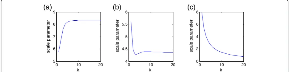
after the iterations are taken some steps. We gain the sequence vector {λk} and find that λk has some proper-ties as follows:
(a) the sequence vector {λk} is monotonically decreasing
as the number of iterationkincreases (see Figure1c);
(b) as the number of iterationkincreases, the sequence
vector {λk} will at first decrease, and then increase
closely toλ0(see Figure1b);
(c) the sequence vector {λk} is monotonically increasing
as the number of iterationkincreases (see
Figure1a).
Therefore, we can obtain the initial value of varying scale parameter by the trend of the sequence vector {λk} as follows:
(1) If the sequence vector {λk} is monotonically
decreasing at first as the number of iterationk
increases, we consider that the random selectedλ0
is contented with the property of (a) or (b). Then,
the initial scale parameterλ1of our proposed
method is equal toλk. Usually,kis equal to 3.
(2) If the sequence vector {λk} is monotonically
increasing as the number of iterationkincreases,
the random selectedλ0is contented with the
property of (c). Then, the initial scale parameter of
our proposed methodλ1¼λ1orλ1=λ0/pwith
the constantp> 1. Usually,p= 2.
In Figure 1, as the example of ‘Barbara’ image, the trends of the sequence vector {λk} are gained when the scale parameterλ0is 8.33, 4.34, and 0.013, respectively.
IRM framework with varying scale parameter
According to the above two sections, our general iterative regularization procedure can be formulated as follows.
ujþ1¼arg min
u∈BVð ÞΩ J uð Þ þ λ0
2 ∥f þvju 2 2 ∥
vjþ1¼vjþf ujþ1 8
<
: ð11Þ
Step 1: We randomly selectλ0. Letu0= 0,v0= 0 and
j= 0, 1, 2. . .
0 10 20
5 6 7 8 9
k
0 10 20
4 4.5 5 5.5 6
k
0 10 20
0 2 4 6 8
k
(a)
(b)
(c)
scale parameter scale parameter scale parameter
(1) According to Equations (11) and (10), we calculate uj+1, vj+1, andλjby the number of iterationj.
Generallyj= 2.
(2) We observe the trend of the sequence vector {λk}.
According to the properties of“Initial scale
parameter”section, we get the initial valueλ1of our
proposed method.
Step 2: Letu0= 0,v0= 0 andk= 1, 2. . .
(1) According to Equation (9) and the initial valueλ1,
we calculate uk+1, vk+1, andλk+1.
(2) We get imageukand stop the iteration when
∥f-u∥k≤σ(as the stopping criterion).
Result and discussion
All solutions to the variational problem were obtained using gradient descent in a standard fashion [21-28]. Now, we use Chambolle Algorithm [8]. The only non-trivial difficulty comes when |∇u|≈0. We fix this, as
is usual, by perturbing J uð Þ ¼
∬
Ω ∇
u
j jdxdy to Jεð Þ ¼u
∬
Ω ffiffiffiffiffiffiffiffiffiffiffiffiffiffiffiffiffiffiffiffiffij∇uj2þε2q
dxdy, where εis a small positive number.
(a)
k=1, PSNR=19.7dB(b)
k=5, PSNR=25.1dB(c)
k=15, PSNR=30dB(d)
k=21, PSNR=28.8dB(e)
k=1, PSNR=25dB(f)
k=2, PSNR=30.2dB(g)
k=3, PSNR=28.3dB(h)
k=5, PSNR=25.4dB0 10 20
0 2 4 6 8 0
0 10 20 30
2 4 6 8
nor
m
2
of
f
and u
||f-u
k||
2noisenorm
0 5 10
0 1 2 3 4
nor
m
2
of
f
and u
||f-u
k||
2noisenorm
(i)
trend of kas k increases(j)
converge of constant k(k)
converge of varying kscale parameter
k k k
To be extent, the ‘stair-casing’effect of this method can be decreased. In our calculations, we too k = 10−12; the step of iteration unit τfor Chambolle Algorithm is 0.2. Without loss of generality, the performance of the denoising algorithms is measured in terms of peak sig-nal-to-noise-ratio (PSNR) [29], which can be defined as follows
PSNR¼10log10 255 2
1
MN
XM
m¼1
XN
n¼1ðfmnumnÞ 2 0
B @
1 C A
ð12Þ
where f is the original image and u is the denoising image.
Convergence analysis
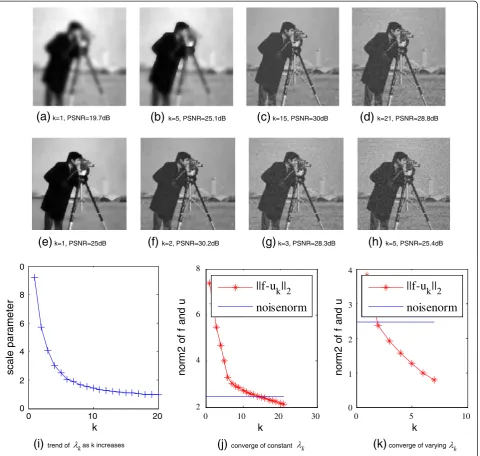
Figures 2 and 3 show the results with constant and vary-ing scale parameter of IRM with ‘cameramen’ image added Gauss noise σ= 20 when λ is smaller and bigger, respectively. In Figure 2, the first row results show that more iteration steps are required to stop criterion with smaller scale parameterλ0= 0.67; the second row results
show that our proposed methods require less iterations to get the optimal denoising results. At first, we used constant scale parameter λ0= 0.67 to iterate three times
and got a sequence vector {λk} decreased in the first image of the third row. According to Equation (11), we got the initial value λ1=λ2= 5.74. The last two plots (i)
and (j) show that∥f−u∥k2decreases monotonically with
the iteration, first dropping below σ at the optimal iter-atek= 12 and 2, respectively. It shows that our proposed
(a)
(b)
(c)
(d)
(e)
(f)
k=2, PSNR=30.2dB(g)
(h)
0 10 20
7.5 8 8.5 9 9.5 10
0 10 20 30
0 0.5 1 1.5 2 2.5 3
||f-uk||2 noisenorm
0 5 10
0.5 1 1.5 2 2.5 3 3.5
||f-u
k||2
noisenorm
(i)
trend of kas k increases(j)
converge of constant k(k)
converge of varying kscale parameter
k k k
norm
2
of f and u
norm
2
of f and u
k=1, PSNR=27.2dB k=2, PSNR=28.7dB k=15, PSNR=23.5dB
k=1, PSNR=26.3dB k=3, PSNR=28.4dB k=5, PSNR=25.6dB
k=21, PSNR=23.5dB
method converge faster than IRM with the constant scale parameter. In Figure 3, as can be seen, with large scale parameter λ0= 10 the original IRM convergences
to the noisy image f quickly, and only one iterative needed to reach the stop criterion. Obviously, the denoising result is not satisfied. However, promising result is obtained by our varying scale parameter strategy where the initial value λ1=λ2= 5.74 according to
Equation (10).
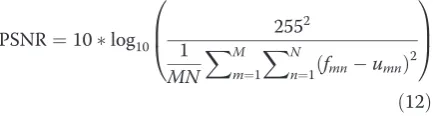
Preserved textures analysis
Figure 4 shows the denoising results of ‘Barbara’image with Gauss white noiseσ= 25.5. The constant scale par-ameterλfor IRM is 1. Compared with the constant scale parameter for IRM in Figure 4c–f, our proposed method can preserved more textures in Figure 4g–j. The last two plots (k) and (l) show that∥f−u∥k2decreases
monoton-ically with the iterations, first dropping below σ at the optimal iterate k= 12 and 2, respectively. It shows that
(a)
original(b)
noisy f(c)
k=1, PSNR=20.1(d)
(e)
k=8, PSNR=24.5(f)
k=12, PSNR=26.1(g)
k=1, PSNR=22.5(h)
k=2, PSNR=25.2(i)
k=3, PSNR=26.2(j)
k=5, PSNR=24.50 5 10 15
2 3 4 5 6 7
nor
m
2 of
f
and u
||f-u
k||2
noisenorm
0 2 4 6 8
1 2 3 4 5 6 7
nor
m
2
of
f
and u
||f-uk||2
noisenorm
(k)
converge of constant k(l)
converge of varying kk k
k=3, PSNR=22.1
our proposed method converges faster than IRM with the constant scale parameter.
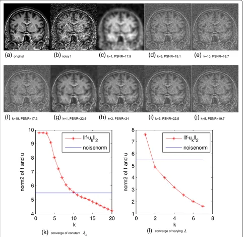
Denoising analysis for MRI coronal brain
The denoising results of MRI coronal brain image with Gauss white noise σ= 53.83 are shown in Figure 5. The constant scale parameterλ for IRM is 1. Compared with the constant scale parameter for IRM in Figure 5c–f, our proposed method can preserve more textures in Figure 5g–j. The last two plots (k) and (l) show that ∥f−u∥k2 decreases monotonically with the iterations,
first dropping belowσat the optimal iteratek= 13 and 3,
respectively. It shows that our proposed method con-verges faster than IRM with the constant scale parameter and has more texture details in the denoised image.
Computational cost analysis
We have made a comparison in terms of computational time (see Tables 1 and 2) by MATLAB 7.1, which is used
(a)
original(b)
noisy f(c)
k=1, PSNR=17.9(d)
k=5, PSNR=15.1(e)
k=10, PSNR=18.7(f)
k=18, PSNR=17.3(g)
k=1, PSNR=22.6(h)
k=2, PSNR=24(i)
k=3, PSNR=22.5(j)
k=5, PSNR=19.70 5 10 15 20
4 5 6 7 8 9 10
norm
2
of
f
and u
||f-u k||2 noisenorm
0 2 4 6 8
1 2 3 4 5 6 7 8
norm
2
of
f
and u
||f-u k||2 noisenorm
(k)
converge of constant(l)
converge of varyingk
k k
Figure 5Denoising results of MRI coronal brain image.
Table 1 Computer time of formula (9)
Computing (9a) Computing the sub-problem (9b)
on a PC equipped with AMD 2.31 GHz CPU and 3 GB RAM. In fact, it should be noted that the term “Fast”is relatively for computing (9a) when compared with com-puting the sub-problem (9b), i.e., in this article even we use the efficient Chambolle Algorithm to solve the sub-problem (9b) and set the inner iterations is 40. To take the results of “Preserved textures analysis” section for denoising‘Barbara’image (256 × 256) as an example, the average time of computing (9b) once is 1.281 s, while that of (9a) once is only 0.026 s. Moreover, combined with fact that the outer iterations of the conventional IRM is 13 while our adaptive IRM is 3, the whole com-putational time of the conventional IRM is 13.708 s while that of our method is 3.136 s. Therefore, we know that our adaptive scheme is really faster than the con-ventional one.
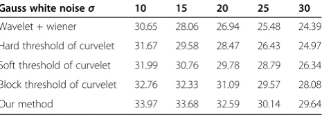
In addition, we have made a comparison between wavelet + wiener, curvelets include hard threshold, soft threshold, and block threshold regulation algorithm and our method. Denoising results of Lena image are shown that our algorithm improves PSNR than traditional method in Table 3.
Conclusion
A novel IRM with adaptive scale parameter is proposed in order to decrease the sensitivity of constant scale par-ameter, optimize the scale parameter adaptively in the IRM, and attain a desirable level of applicability for image denoising. We replace the classic regularization item and deduce the equation of the adaptive scale parameter, be-cause we know that the scale parameter is smaller, the number of the iteration will enhance by IRM. Then, the rule of varying scale parameter by the trend of the sequence vector is attained. A new iterative scale param-eterλis obtained according to the trend of the sequence vector. In general, we can get the initial scale parameter λ just using three steps of iteration. We have seen with practical examples that our proposed method can reduce
the number of iterations. Thus, a fast and robust method is got.
Appendix 1
A constrained problem is defined as
minF Xð Þ s:t:NTXb≥0
ð13Þ
We know that the constraint equation is NTX−b= 0. The basic assumption is thatX lies in the subspace tan-gent to the active constraints, i.e., Xi+1=Xi+αS, where
S is the direction with the most negative directional de-rivative and α is the iterative step length, both Xi and
Xi+1 satisfy the constraint equations. Therefore, we
obtain
NTS¼0 ð14Þ
If we want the steepest descent direction satisfying Equation (14), we can pose the problem as
minST∇F s:t:NTS¼0 andSTS¼1
ð15Þ
The Euler–Lagrange equation (15) has the formulation
L Sð ;λ;μÞ ¼ST∇FSTNλμ STS1 ð16Þ
The derivative ofLwith respect toSis
∂L
∂S¼∇FNλ2μS¼0 ð17Þ
Recall that NTS= 0 in Equation (14) and multiplying Equation (17) byNT, we get
NT∇FNTNλ¼0 ð18Þ
Therefore, we get the value
λ¼NT∇F
NTN ð19Þ
So, the proposition holds.
Appendix 2
In this article, we want to solve the question
ukþ1¼arg min
uεBVð ÞΩ
∬
Ωj∇ujdxdyþλ
2∥f þvku 2 2 ∥
ð20Þ Table 2 Computer time of our method and the
conventional IRM
Our method The conventional IRM
Computational time 3.136 s 13.708 s
Table 3 A variety of image denoising algorithms are compared for Lena image
Gauss white noiseσ 10 15 20 25 30
Wavelet + wiener 30.65 28.06 26.94 25.48 24.39
Hard threshold of curvelet 31.67 29.58 28.47 26.43 24.97
Soft threshold of curvelet 31.99 30.76 29.78 28.79 26.34
Block threshold of curvelet 32.76 32.33 31.09 29.57 28.08
It is equivalent to
ukþ1¼arg min
uεBVð ÞΩ λ1
∬
Ωj∇ujdxdyþ 12∥f þvku 2 2 ∥
ð21Þ
whereλ1¼1
λ. Then, Equation (21) is rewritten to
min
uεBVð ÞΩ
1
2∥f þvku 2 2 ∥
s:t:
∬
Ω ∇u
j jdxdy≥0 8 > > > < > > > : ð22Þ Since
∬
Ω j∇ujdxdy¼∥∇u1∥≈
ffiffiffiffiffiffiffiffiffiffiffiffiffiffiffiffiffiffiffiffi ∥∇u 2
1 ∥þε
p
¼< ∇∇u
ffiffiffiffiffiffiffiffiffiffiffiffiffiffiffi ∥∇u2
1
∥ þε
p ;u>, we let ∇ffiffiffiffiffiffiffiffiffiffi∇u ∇u2
1þε
p be approximated by ∇∇u
k
ffiffiffiffiffiffiffiffiffiffiffiffiffiffiffiffi ∥∇uk∥21þε
p , and let u¼X;b¼0;N¼ ffiffiffiffiffiffiffiffiffiffiffiffiffiffiffiffi∇∇uk
∥∇uk∥21þε
p and
u
ð Þ ¼1
2∥f þvku∥22, we have
∬
Ω j∇ujdxdy¼¼N
Tu≥0,
then according to Appendix 1, we obtain
λ1¼
∬
Ω∇ 1
∇uk
j j∇uk
ukf vk
ð Þdxdy
∬
Ω∇1 ∇uk
j j∇uk
∇ 1 ∇uk
j j∇uk
dxdy
ð23Þ
Therefore, we obtain the parameter
λ¼ 1 λ1¼
∬
Ω∇1 ∇uk
j j∇uk
∇ 1
∇uk
j j∇uk
dxdy
∬
Ω∇1 ∇uk
j j∇uk
ukf vk
ð Þdxdy
ð24Þ
So, the proposition holds.
Competing interests
The authors declare that they have no competing interests.
Acknowledgment
This study was supported by the National Natural Science Foundation of China under the Grant nos. 60702069, 30300443 and 61105035; the Research Project of Department of Education of Zhejiang Province, China under the Grant no. 20060601; The Science Foundation of Zhejiang Sci-Tech University of China under the Grant no. 0604039-Y; the Natural Science Foundation of Zhejiang Province of China under the Grant no. Y1080851 and Y12H290045; the Research Project of 2011 overseas students of Zhejiang Province of China under the Grant no. 1104707-M; Qianjiang talents project of Science and Technology Department of Zhejiang province of China under the grant no. 2012R10054.
Author details
1
Lab of Intelligence Detection and System, School of Information Science and Technology, Zhejiang Sci-Tech University, Hangzhou, China.2School of Life Science and Technology, Shanghai Jiao Tong University, Shanghai 200240, China.
Received: 23 April 2012 Accepted: 11 September 2012 Published: 16 October 2012
References
1. L Rudin, S Osher, E Fatemi, Nonlinear total variation based noise removal algorithms. Physica D60, 259–268 (1992)
2. R Devore, B Jawerth, B Lucier, Image compression through wavelet transform coding. IEEE Trans. Inf. Theory38, 719–746 (1992)
3. DL Donoho, De-noising by soft-threshold. IEEE Trans. Inf. Theory41(3), 613– 627 (1995)
4. K Dabov, A Foi, V Katkovnik, K Egiazarian, Image denoising by sparse 3-D transform-domain collaborative filtering. IEEE Trans. Image Process.16, 2080–2095 (2007)
5. R Yan, L Shao, SD Cvetkovic, J Klijn, Improved nonlocal means based on pre-classification and invariant block matching. IEEE/OSA J. Disp. Technol. 8(4), 212–218 (2012)
6. S Osher, A Solè, L Vese, Image decomposition and restoration using total variation minimization and the H-1 norm. SIAM J. Multiscale Model. Simulat. 1(3), 349–370 (2003)
7. M Burger, G Gilboa, S Osher, JJ Xu, Nonlinear inverse scale space methods. Commun. Math. Sci.4(1), 175–208 (2006)
8. A Chambolle, R DeVore, NY Lee, B Lucier, Nonlinear wavelet image processing: variational problems, compression, and noise removal through wavelet shrinkage. IEEE Trans. Image Process.7(3), 319–335 (1998) 9. A Chambolle, BJ Lucier, Interpreting translation-invariant wavelet shrinkage
as a new image smoothing scale space. IEEE Trans. Image Process. 10, 993–1000 (2001)
10. G Steidl, J Weickert, T Brox, P MraZek, M Welk, On the equivalence of soft wavelet shrinkage, total variation diffusion, total variation regularization, and SIDEs. SIAM J. Numer. Anal.42(2), 686–713 (2004)
11. J Xu, S Osher, Iterative regularization and nonlinear inverse scale space applied to wavelet-based denoising. IEEE Trans. Image Process. 16(2), 534–544 (2007)
12. Y. Meyer,Oscillating Patterns in Image Processing and Nonlinear Evolution Equations(American Mathematical Society, Boston, 2002)
13. S Osher, M Burger, D Goldfarb, J Xu, W Yin, An iterative regularization method for total variation based image restoration. Multiscale Model. Simulat.4, 460–489 (2005)
14. L Bregman, The relaxation method of finding the common points of convex sets and its application to the solution of problems in convex programming. U.S.S.R. Comput. Math. Math. Phys.7, 200–217 (1967) 15. BB Hao, M Li, XC Feng, Wavelet iterative regularization for image restoration
with varying scale parameter. Signal Process. Image Commun.23(6), 433– 441 (2008)
16. B Liu, K King, M Steckner, J Xie, J Sheng, L Ying, Regularized sensitivity encoding (SENSE) reconstruction using Bregman iterations. Magn. Reson. Med.61(1), 145–152 (2009)
17. A Chambolle, An algorithm for total variation minimization and applications. J. Math. Imag. Vis.20, 89–97 (2004)
18. L Vese, S Osher, Modeling textures with total variation minimization and oscillating patterns in image processing. J. Sci. Comput.19, 553–572 (2003) 19. T Weissman, E Ordentlich, G Seroussi, S Verdu, M Weinberger, Universal
discrete denoising: known channel. IEEE Trans. Inf. Theory51, 5–28 (2005) 20. P Perona, J Malik, Scale space and edge detection using anisotropic
diffusion. IEEE Trans. Pattern Anal. Mach. Intell.12, 629–639 (1990) 21. T Goldstein, S Osher, The split Bregman method for L1-regularized
problems. SIAM J. Imag. Sci.2(2), 323–343 (2009)
22. W Yin, S Osher, D Goldfarb, J Darbon, Bregman iterative algorithms for l1-minimization with applications to compressed sensing. SIAM J. Imag. Sci. 1, 142–168 (2009)
23. L He, TC Chang, S Osher, T Fang, P Speier,MR image reconstruction by using the iterative refinement method and nonlinear inverse scale space methods, 2006. Technical Report CAM Report 06–35, UCLA
24. E Esser,Applications of Lagrangian-based alternating direction methods and connections to split Bregman, 2009. CAM Report 09–31, UCLA
25. Y Wang, J Yang, W Yin, Y Zhang, A new alternating minimization algorithm for total variation image reconstruction. SIAM J. Imag. Sci.
1(3), 248–272 (2008)
27. J Ma, DF Le, Deblurring from highly incomplete measurements for remote sensing. IEEE Trans. Geosci. Remote Sensing (GeoRS)3(47), 792–802 (2009) 28. G Gilboa, N Sochen, YY Zeevi, Texture preserving variational denoising
using an adaptive fidelity term, inProc VLSM Nice, France1, 2003, pp. 137–144
29. L Shao, H Zhang, G de Haan, An overview and performance evaluation of classification-based least squares trained filters. IEEE Trans. Image Process. 17, 1772–178 (2008)
doi:10.1186/1687-6180-2012-222
Cite this article as:Liet al.:A parameter-adaptive iterative regularization model for image denoising.EURASIP Journal on Advances in Signal Processing20122012:222.
Submit your manuscript to a
journal and benefi t from:
7Convenient online submission
7Rigorous peer review
7Immediate publication on acceptance
7Open access: articles freely available online
7High visibility within the fi eld
7Retaining the copyright to your article