Stochastic analysis of neural network modeling and identification of nonlinear memoryless MIMO systems

(1)

R E S E A R C H

Open Access

Stochastic analysis of neural network modeling

and identification of nonlinear memoryless MIMO

systems

Mohamed Ibnkahla

*

Abstract

Neural network (NN) approaches have been widely applied for modeling and identification of nonlinear multiple-input multiple-output (MIMO) systems. This paper proposes a stochastic analysis of a class of these NN algorithms. The class of MIMO systems considered in this paper is composed of a set of single-input nonlinearities followed by a linear combiner. The NN model consists of a set of single-input memoryless NN blocks followed by a linear combiner. A gradient descent algorithm is used for the learning process. Here we give analytical expressions for the mean squared error (MSE), explore the stationary points of the algorithm, evaluate the misadjustment error due to weight fluctuations, and derive recursions for the mean weight transient behavior during the learning process. The paper shows that in the case of independent inputs, the adaptive linear combiner identifies the linear combining matrix of the MIMO system (to within a scaling diagonal matrix) and that each NN block identifies the corresponding unknown nonlinearity to within a scale factor. The paper also investigates the particular case of linear identification of the nonlinear MIMO system. It is shown in this case that, for independent inputs, the adaptive linear combiner identifies a scaled version of the unknown linear combining matrix. The paper is supported with

computer simulations which confirm the theoretical results.

Keywords:Nonlinear system identification, Neural networks, Gradient descent, Statistical analysis

Introduction

Neural network [1] approaches have been extensively used in the past few years for nonlinear MIMO system modeling, identification and control where they have shown very good performances compared to classical techniques [2-6].

If these NN approaches are to be used in real systems, it is important for the algorithm designer and the user to understand their learning behavior and performance cap-abilities. Several authors have analyzed NN algorithms during the last two decades which considerably helped the neural network community to better understand the mechanisms of neural networks [1,7-15]. For example, the authors in [13] have studied a simple structure con-sisting of two inputs and a single neuron. The authors in [8] studied a memoryless single-input single-output (SISO) system identification model for the single neuron

case. In [9] the authors proposed a stochastic analysis of gradient adaptive identification of nonlinear Wiener sys-tems composed of a linear filter followed with a Zero-memory nonlinearity. The model was composed of a lin-ear adaptive filter followed by an adaptive parameterized version of the nonlinearity. This study has been later generalized [16] for the analysis of stochastic gradient tracking of time-varying polynomial Wiener systems. In [12] the author analyzed NN identification of nonlinear SISO Wiener systems with memory for the case where the adaptive nonlinearity is a memoryless NN with an ar-bitrary number of neurons. The case of a nonlinear SISO Wiener-Hammerstein system (i.e., an adaptive filter fol-lowed by an adaptive Zero-memory NN folfol-lowed by an adaptive filter) has been analyzed in [11].

This paper deals with a typical class of nonlinear MIMO systems (Figure 1) which is composed of M

inputs, M memoryless nonlinearities, a linear combiner, andLoutputs. This corresponds, for example, to MIMO channels used in wireless terrestrial communications

Correspondence:[email protected]

Electrical and Computer Engineering Department, Queen_’s University, Kingston, Ontario K7L 3N6, Canada

(2)

[17-22], satellite communications [23,24], amplifier mod-eling [25], control of nonlinear MIMO systems [6], etc. Recently, a neural network approach has been proposed to adaptively identify the overall input–output transfer function of this class of MIMO systems and to characterize each component of the system (i.e., the memoryless nonlinearities and the linear combiner) [4]. The proposed NN model is composed of a set of mem-oryless NN blocks followed by an adaptive linear com-biner. Each part of the adaptive system aims at identifying the corresponding part in the unknown MIMO system. The algorithm has been successfully ap-plied to system modeling, channel tracking, and fault detection.

The purpose of this paper is to provide a stochastic analysis of NN modeling of this class of MIMO systems. The paper provides a general methodology that may be used to solve other problems in stochastic NN learning analysis. The methodology consists of splitting the study into simple structures, before studying the complete structure. Here, as a first step we start by analyzing a simple linear adaptive MIMO scheme (consisting of an adaptive matrix) that identifies the nonlinear MIMO sys-tem (i.e., problem of linear identification of a nonlinear MIMO system). Then we analyze a nonlinear adaptive system in which the nonlinearities are assumed to be known and frozen during the learning process, only the linear combiner is made adaptive. Finally, the complete adaptive scheme is analyzed taking into account the insights given by the analysis of the simpler structures. In our analytical approach, we derive the general formu-las and recursions, which we apply to a case study that we believe is illustrative to the reader.

The paper is organized as follows. The problem state-ment is given in Section 2. The study of the simple

structures is detailed in Section 3. Section 4 presents the analysis for the complete structure. Simulation results and illustrations are given in Section 5. Finally, conclu-sions and future work are given in Section 6.

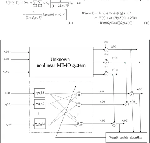
Problem statement Nonlinear MIMO system

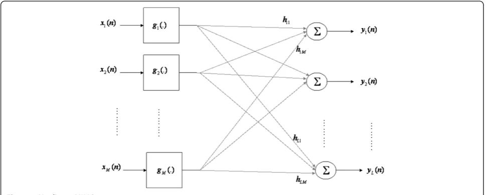
The class of nonlinear MIMO systems discussed in this paper is presented in Figure 1. Each inputxi(n) (i =1,. . .,

M) is nonlinearly transformed by a memoryless nonlinear-ity gi (.). The outputs of these nonlinearities are then linearly combined by an L×Mmatrix H =[hji] (assumed in this paper to be constant). Matrix His defined by the unknown system to be identified. For example, in wireless MIMO communication systems, M is the propagation matrix representing the channel between M transmitting antennas andLreceiving antennas.

Thejthoutput of the MIMO system is expressed as:

yjð Þ ¼n XM

i¼1

hjið Þgn iðxið Þn Þ þNjð Þn ð1Þ

whereNjis a white Gaussian noise with varianceσ02.

Let X nð Þ¼ x1ð Þn x2ð Þn . . .xMð Þn t;g X nð ð ÞÞ¼

g1ðx1ð ÞnÞ ½

g2ðx2ð ÞnÞ. . .gMðxMð ÞnÞt;Y nð Þ ¼ y1ð Þny2ð Þn . . .yLð Þn t;

and N nð Þ ¼ N1ð ÞN2n ð Þn . . .NLð Þn t:

The system input–output relationship can be expressed in a matrix form as:

Y nð Þ ¼Hg X nð ð ÞÞ þN nð Þ: ð2Þ

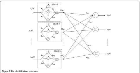
Neural Network identification structure and algorithm

(3)

neurons and a scalar output. The output of the kthblock is expressed as:

NNkð Þ ¼n XN

i¼1

ckif að kixkð Þ þn bkiÞ;k¼1; ::::;M ð3Þ

Where fis the NN activation function. aki, cki, bki are, respectively, the input weight, bias term, and output weight of the ith neuron in the kth block. The output

NNkof thekthblock is connected to thejthoutput of the system through weightwjk. The systemjthoutput is then

expressed as:

sjð Þ ¼n XM

k¼1

wjkNNkð Þn;j¼1; ;L ð4Þ

Weights wjk will be represented by an LxM matrix:

W = [wjk].

Let S nð Þ¼ s1ð Þs2n ð Þn . . .sLð Þn t and NN nð Þ¼

NN1ð Þn ½ NN2ð Þn . . .NNMð Þn t:

Equations (4) can then be expressed in a matrix form as:

S nð Þ ¼WNN nð Þ: ð5Þ

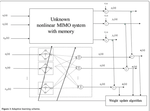
For the learning process, the NN parameters are updated so that to minimize the sum of the squared errors between the unknown system outputs and the corresponding outputs of the model (Figure 3):

e nð Þ

k k2_¼XL

j¼1

e2_jð Þn: ð6Þ

Here ejð Þ ¼n yjð Þ n sjð Þn and e nð Þ ¼½e1ð Þe2n ð Þn . . .

eLð Þn t:

The gradient descent recursions for weight adaptation are:

W nð þ1Þ ¼W nð Þ þ2μe nð ÞNNtð Þn ð7Þ

ckiðnþ1Þ ¼ckið Þ þn 2μf að kixkð Þ þn bkiÞ XL

l¼1

wlkelð Þn

ð8Þ

akiðnþ1Þ ¼akið Þ þn 2μckixkð Þn f

0

akixkð Þn

ð þbkiÞ

XL

l¼1wlkelð Þn ð9Þ

bkiðnþ1Þ ¼bkið Þþn 2μckif

0

akixkð Þþbn ki

ð Þ

XL_l_¼1wlkelð Þn ð10Þ

whereμ is a small positive constant and f0ðÞ represents the derivative:f0ð Þ ¼x @f x_@ð Þ_x :

Case study

(4)

In this case study, the inputs xi (n) will be assumed uncorrelated Zero-mean Gaussian variables with variance

σ2

xi. The NN activation function will be taken as theerf function. The unknown nonlinear transfer functions are taken from a family of nonlinear functions of the form

gið Þ ¼x αixexp βix

2 2

, where αi and βi are positive

con-stants. These nonlinear functions are reasonable models for amplitude conversions of nonlinear high power amplifiers (HPA) used in digital communications [12,25,26]. Note that other nonlinear functions may be considered, however, explicit closed-form solutions of the different derivations may not be possible.

Study of simplified structures: Linear adaptation

Before analyzing the full structure, we will analyze the following simplified schemes which will help us under-stand the complete structure:

1. The adaptive system is composed of an adaptive

linear combinerW(Section 3.1).

2. The adaptive system is composed ofWand scaled

versions of the unknown nonlinearities (Section 3.2).

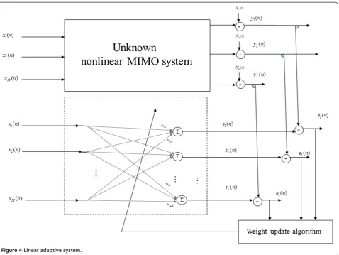
Linear adaptive system

This section studies the linear adaptive system that tries to model the nonlinear MIMO system (Figure 4):

Mean weight behavior and Wiener solution

Since matrix W is linear, it will not be able to identify the nonlinear blocks. However, we will see that it is able to identify matrix H to within a diagonal scaling matrix if the inputs are Zero-mean and independent.

The gradient descent update of matrixWis expressed as:

W nð þ1Þ ¼W nð Þ þ2μe nð ÞXtð Þn ¼W nð Þ þ2μððHgX nð Þ þN nð Þ

W nð ÞX nð ÞÞXt_{ð Þ}_n _ð₁₁_Þ

Averaging both sides of (11) and using the standard LMS assumption of smallμ[10], we obtain:

E W nð ð þ1ÞÞ E W nð ð ÞÞ þ2μ HRg Xð ÞX

E W nð ð ÞÞRXXÞ

¼E W nð ð ÞÞðI2μRXXÞ þ2μHRg Xð ÞX

ð12Þ WhereRXX¼E XXð tÞ;Rg Xð ÞX ¼E g Xð ð ÞXtÞ:

(5)

By setting the updating gradient term to Zero, it can be shown that this equation has a single stationary point (Wiener solution [10]) which is expressed by:

W ¼W0¼HU where U¼Rg Xð ÞXR1XX ð13Þ

Following Equation (12), the mean weights can be expressed as a function of the initial condition as:

E W nð ð ÞÞ ¼Wð Þ0 ðI2μRXXÞn

þ2μHRg Xð ÞX Xn1

p¼0

I2μRXX

ð Þp _ð

14Þ

If μ is sufficiently small, the first term converges to 0 and the second term converges toHRg Xð ÞXR1XX.

Hence, the mean weights converge to the Wiener solution:

Wð Þ ¼1 W0¼HRg Xð ÞXR1XX ð15Þ

It can be easily shown that the stability condition onμ is [10]:

0<μ< 1

λmax ð

16Þ

where λmax is the largest eigenvalue of the covariance

matrixRXX.

Note that for Zero-mean independent inputs,Uis a di-agonal matrix:

U¼Rg Xð ÞXR1XX

¼

E g½ 1ð Þx1 x1 σ2

x1

0. . . 0

0 E g2½ ð Þx2x2

σ2

x2

. . .

0 0. . . E g½ Mð ÞxM xM

σ2

xM 2

6 6 6 6 6 6 6 6 4

3 7 7 7 7 7 7 7 7 5

ð17Þ

(6)

expected, the scaling matrix reduces to the identity matrix ifgk(xk) =xk.

Application to the case study:

For the particular nonlinear functions given in the case study (see Section 2.3), it is easy to show:

E xð ið Þgn iðxið Þn ÞÞ ¼ αiσxi

2

1þβ_iσxi2

3

2 and

E g_i2ðxið ÞnÞ

¼ α2iσxi

2

1þ2β_iσxi2

3

2 ð

18Þ

The mean weight transient recursions are expressed as:

E wjkðnþ1Þ

¼E wjkð Þn

12μσ2_x_k

þ2μhjk

αkσ2xk

1þβ_kσ2

xk

3

2

ð19Þ

MatrixUreduces to the following diagonal matrix:

U¼

α1

1þβ₁σ2

x1

3

2

0. . . 0

0 α2

1þβ₂σ2

x2

3

2 . . .

0 0. . . αM

1þβ_Mσ2

xM

3

2

2 6 6 6 6 6 6 6 6 6 6 4

3 7 7 7 7 7 7 7 7 7 7 5

ð20Þ

Transient MSE and Wiener MSE

The transient MSE is determined by:

Eke nð Þk2¼EkHg X nð ð ÞÞ þN nð Þ W nð ÞX nð Þk2

¼X

L

j¼1

E e2_jð Þn

h i

ð21Þ

where:

E e 2_jð Þn¼E Hjg X nð ð ÞÞ þNjð Þ n Wjð Þn X nð Þ

2

ð22Þ

where Wjð Þ ¼n wj1ð Þn wj2ð Þn . . . wjMð Þ n t and Hj¼

hj1hj2. . .hjMt:

Using the independence of noise and weights at time

n, we get:

E e _j2ð Þn¼σ2₀þE ðHjg X nð ð ÞÞ Wjð Þn X nð Þ

2

¼σ2

0þHjtRg Xð Þg Xð ÞHj2HjtRg Xð ÞXE Wjð Þn

þE Wjð ÞnRXXWjtð Þn

ð23Þ

The total MSE is therefore expressed as:

Eke nð Þk2¼Lσ2₀þX

L

j¼1

H_jtRg Xð Þg Xð ÞHj

2H_jtRg Xð ÞXE Wjð Þn

þE W_jtð ÞnRXXWjð Þn

: ð24Þ

Wiener MSE:

The Wiener MSE, ζ0¼E keW0ð Þnk 2

, is the minimum MSE that can be reached by the system if W is equal to the Wiener solutionW0=HU. It can be easily shown that:

ζ0¼E keW0ð Þn k 2

¼Lσ2₀þEkHg X nð ð ÞÞ W0X nð Þk2

¼Lσ2₀þEkH g X nð ð ð ÞÞ UX nð ÞÞk2 ð25Þ

It is clear from this equation that if the unknown func-tions are linear, then the Wiener MSE reduces to the noise power. The MSE is always larger than ζ0 because

of the misadjustment error introduced by the weight fluctuations.

Now we can write the MSE as a function of the Wiener MSE:

Eke nð Þk2¼EkH g X nð ð ð ÞÞ þN nð ÞW nð ÞX nð ÞÞk2 ¼E keW0ð Þ n ðW nð Þ W0ÞX nð Þk

2

ð26Þ Let the instantaneous deviation of the matrix weights with respect to the Wiener solution be denoted by:

V nð Þ ¼ vjkð Þn

¼W nð Þ W0: ð27Þ

We have:

Eke nð Þk2¼E keW0ð Þ n V nð ÞX nð Þk 2

: ð28Þ

This expression is similar to that of the well-known LMS algorithm [10], and can be evaluated as the sum of the minimum error and excess error (or misadjustment) as:

Eke nð Þk2¼ζ0þ

XL

j¼1

tr RXXKVjVjð Þn

ð29Þ

where Vjð Þ ¼n vj1vj2. . .vjM

t

and KVjVjð Þ ¼n E Vjð Þn

(7)

The misadjustment is expressed as:

Δð Þ ¼n tr RXX XL

j¼1

RVjVjð Þn !

: ð30Þ

At the convergence, we have:

Ekeð Þ1k2¼ζ0þΔð Þ1: ð31Þ

Derivation of the misadjustment:

From Equation (11) it is easy to show that the weight fluctuations follow the recursion:

V nð þ1Þ ¼V nð Þ þ2μðeW0ð Þ n V nð ÞX nð ÞÞX

t_{ð Þ}_n

ð32Þ Taking the mean of this equation and applying the or-thogonality principle between the input vector and the Wiener error, we get:

E V nð ð þ1ÞÞ ¼E V nð ð ÞÞð12μRXXÞ ð33Þ Thus, as expected, ifμis sufficiently smallE(V(n)) con-verges to 0.

Similarly, for each vectorVjwe can obtain the follow-ing recursion:

Vjðnþ1Þ ¼Vjð Þ þn 2μ eW0jð Þ n X

t_{ð Þ}_n _V jð Þn

X nð Þ Þ ð34Þ The evaluation of the covariance matrix of the weight fluctuations is obtained by multiplying both sides of Equation (34) byVt

jðnþ1Þand averaging:

KVjVjtðnþ1Þ ¼KVjtVjtð Þ n 2μRXXKVjVjð Þn

2μKVjVjð ÞRn XX

þ2μE eW0jð Þn XV

t

jðI2μXXtÞ

h i

þ2μE eW0jð ÞXVn

t

jðI2μXXtÞ

h it

þ4μ2_{E XX}t_K VjVjXX

t

þ4μ2E e2_W₀_jð Þn XXt

h i

ð35Þ

These expectations are derived in Appendix III, which yields:

2μKVjVjð ÞnRXX

þ4μ2 E H_jtg Xð ÞXE V_jtð Þn

XXt

h i

þtr RXXW0E Vjtð Þn

RXX

þRXXW0E Vjtð Þn

RXX

XXt

h i

RXX

þRXXW0E Vjtð Þn

RXX t

þ4μ2 tr RXXKVjVjð Þn

RXX

þ2RXXKVjVjð ÞnRXX

þ4μ2 E g Xð Þgtð ÞX HjHjtXXt

h i

þσ2

0RXXtr RXXW0tjW0tj

RXX

2RXXW0tjW0tjRXX

ð36Þ

Taking into account that E(Vj(∞)) = 0, KVjVj can be

obtained by solving the following equation:

RXXKVjVjð Þþ1 KVjVjð Þ1RXX2μtr RXXKVjVjð Þ1

RXX

4μRXXKVjVjð ÞR1 XX

¼2μ E g Xð Þgtð ÞX HjHjtXXt

h i

þ2μσ2₀RXX h

2μtr RXXW0tjW0tj

RXX4μRXXW0tjW0tjRXX i

ð37Þ

This expression holds for any input signal. It can be simplified ifRXX ¼σ2xI. In this case we have:

tr RXXKVjVjð Þ1

¼μσ 2

0σ2xMþtr E g Xð Þgtð ÞHX jHjtXXt

σ4

xðMþ2Þtr W0jW0tj

1μσ2

xðMþ2Þ

ð38Þ

It is now easy to determine the total misadjustment:

Δð Þ ¼1 XL

j¼1

tr RXXKVjVjð Þ1

¼μ

σ2

0σ2xMLþtr E g Xð Þgtð ÞX PL j¼1

HjHjtXXt !

" #

σ4

xðMþ2Þtr W0W0t

1μσ2

xðMþ2Þ

(8)

Note that, as expected, in the case of linear functions Δ(∞) reduces to:

Δð Þj1 g Xð Þ¼X¼

μσ2 0σ2xML 1μσ2

xðMþ2Þ

: ð40Þ

The additional terms are due to the nonlinearities and they should be calculated specifically for each nonlinearity.

Application to the case study: The MSE is expressed as:

Eke nð Þk2¼Lσ02þ

XL

j¼1 XM

k¼1 αkσ2xk

αk 1þ2β_iσxk2

3

2 h2_jk

2 4

2

1þβ_kσxk2

3

2

hjkwjkð Þ þn w2jkð Þn 3 5

ð41Þ

The Wiener MSE is expressed in this case as:

ζ0¼Lσ02þ

XM

i¼1

α2

iσ2xi

1þ2β_iσxi

2

3

2₁

1þβ_iσxi2

3

XL

j¼1

h2_ji

ð42Þ

Adaptive W, the nonlinearities are frozen and known with scale factors

In this section, matrix W is adaptive, the nonlinearities are frozen and known with scale factors (Figure 5).

Mean weight behavior and stationary points

The gradient descent update of matrix W is expressed as:

W nð þ1Þ ¼W nð Þ þ2μe nð ÞΩg X nð ð ÞÞt ¼W nð Þ þ2μ½ðHg X nð ð ÞÞ þN nð Þ

W nð ÞΩg X nð ð ÞÞΩg X nð ð ÞÞt ð43Þ

(9)

whereΩ¼

η1 0 0

0 . . . 0

0 η_M

2 4

3 5.

Averaging both sides of (43) and using the standard LMS assumption of smallμ, we obtain:

E W nð ð þ1ÞÞ E W nð ð ÞÞ þ2μ HΩRg Xð Þg Xð Þ

E W nð ð ÞÞΩ2_R

g Xð Þg Xð Þ ¼E W nð ð ÞÞ I2μΩ2Rg Xð Þg Xð Þ

þ2μHΩRg Xð Þg Xð Þ ð44Þ These recursions have a single stationary point (Wiener solution) which is:

W ¼W0¼HΩ1 ð45Þ

Following Equation (44), the mean weight behavior can be expressed as function of the initial condition as:

E W nð ð ÞÞ¼Wð Þ0 I2μΩ2Rg Xð Þg Xð Þ

n

þ2μHΩRg Xð Þg Xð Þ

Xn1

p¼0

I2μΩ2Rg Xð Þg Xð Þ

p

ð46Þ

Hence, if μ is sufficiently small, it can be shown that the mean weights converge to the Wiener solution:

Wð Þ ¼1 W0¼HΩ1: ð47Þ

The stability condition onμis: 0<μ< 1

λmax

Where λmaxis the largest eigenvalue of the covariance

matrixΩ2Rg(X)g(X).

Thus, if each nonlinear functiongk (.) is known with a scaling factor ηk, then weights hjk will be identified by wjk(to the inverse of the scaling factor).

MSE

We have:

Eke nð Þk2¼E Hg X nðk ð ð ÞÞ þN nð Þ W nð ÞΩg X nð ð ÞÞk2

¼XL

j¼1

E e2_jð Þn

h i

ð48Þ

where:

E e2_jð Þn

¼E Hjg X nð ð ÞÞ þNjð Þn

Wjð Þn Ωg X nð ð ÞÞ2

ð49Þ

Using the independence of noise and weights at time

n, we obtain:

E e2_jð Þn

¼σ2

0þE HjΩWjð Þn

g X nð ð ÞÞ

2

¼σ2

0þHjtRg Xð Þg Xð ÞHj

2H_jtΩRg Xð Þg Xð ÞE Wjð Þn

þE W_jtð Þn Ω2Rg Xð Þg Xð ÞWjð Þn

The MSE is therefore expressed as:

Eke nð Þk2¼Lσ2₀þX

L

j¼1

HjtRg Xð Þg Xð ÞHj

2HjtΩRg Xð Þg Xð ÞE Wjð Þn

þE W_jtð ÞnΩ2Rg Xð Þg Xð ÞWjð Þn

ð50Þ

Wiener MSE:

The Wiener MSE can be easily expressed as:

ζ0¼E e2W0ð Þn

¼Lσ2₀þEkðHW0ΩÞg X nð ð ÞÞk2¼Lσ2₀ ð51Þ Therefore the Wiener MSE is equal to the noise floor: There are no terms due to the nonlinearities. This is expected since the nonlinearities are known with a scal-ing matrix Ω (we have seen that the scaling matrix is canceled byW0sinceW0= HΩ-1).

Let Z (n) = Ω g(X(n)), we can then express the MSE as a function ofζ0, the weight fluctuation vector V(n) =

W(n)–W0, and Z(n):

Eke nð Þk2¼E keW0ð Þ n ðW nð Þ W0ÞZ nð Þk 2

¼ζ0þE kV nð ÞZ nð Þk2

¼ζ0þ

XL

j¼1

tr RZZKVjVjð Þn

ð52Þ

Similarly to Equation (29), the misadjustment is expressed as:

Δð Þ ¼n tr RZZ XL

j¼1

KVjVjð Þn !

: ð53Þ

The steady state MSE is then expressed as:

Ekeð Þ1k2¼ζ0þΔð Þ1: ð54Þ

Derivation of the misadjustment:

It is easy to show that the weight fluctuations follow the recursion:

V nð þ1Þ ¼V nð Þ þ2μðeW0ð Þ n V nð ÞZ nð ÞÞZ

t_{ð Þ Þ}_n _:

(10)

Taking the mean of this equation and applying the or-thogonality principle between the input vector and the Wiener error, we obtain:

E V nð ð þ1ÞÞ ¼E V nð ð ÞÞ ð12μRZZÞ: ð56Þ Thus, as expected, if μ is sufficiently small, E(V(n)) converges to 0.

For each vectorVjwe have similar recursions:

Vjðnþ1Þ ¼Vjð Þ þn 2μ eW0jð Þ n Z nð Þ

t

Vjð Þn

Z nð Þ Þ: ð57Þ

The evaluation of the covariance matrix of the weight fluctuations is obtained by multiplying both sides of Equation (57) byVt

jðnþ1Þand averaging:

KVjVjtðnþ1Þ

¼KVt jV

t

jð Þ n 2μRZZKVjVjð Þ n 2μKVjVjð ÞRn ZZ

þ2μE eW0jð ÞZ nn ð ÞV

t

j I2μZ nð ÞZ nð Þ t

h i

þ2μE eW0jð ÞZ nn ð ÞV

t

j I2μZ nð ÞZ nð Þ t

h it

þ4μ2E Z nð ÞZ nð ÞtKVjVjZ nð ÞZ nð Þ t

þ4μ2E e2_W₀_jð ÞZ nn ð ÞZ nð Þt

h i

ð58Þ

In a similar way as in Appendix III, KVjVj (∞) can be obtained by solving the following equation:

RZZKVjVjð Þ þ1 KVjVjð Þ1RZZ2μtr RZZKVjVjð Þ1

RZZ

4μRZZKVjVjð ÞR1 ZZ

¼2μ E g Xð Þgtð ÞX HjHjtZZt

h i

þ2μσ2₀RZZ h

2μtr RZZW0tjW0tj

RZZ4μRZZW0tjW0tjRZZ i

ð59Þ

This expression can not be further simplified because

RZZis not necessarily of the formσ2

zI.

Therefore, tr(RZZ KVjVj (∞)) should be calculated for each nonlinearity and for eachΩ.

It is interesting to study the case where nonlinearities are known with the same scaling factor, i.e., Ω =ηI. In this case, and if the input vectors are independent and the outputs of the nonlinearities are Zero-mean and of equal varianceσ2

g, we have:

tr RZZKVjVjð Þ1

¼μ σ20η2σ2gM 1μη2_σ2

gðMþ2Þ

ð60Þ

As expected, the total misadjustment reduces to:

Δð Þ¼1 XL

j¼1

tr RZZKVjVjð Þ1

¼μ σ

2 0η2σ2gML 1μη2σ2

gðMþ2Þ :

ð61Þ

Here the value of the misadjustment is similar to that of linear identification of a linear system (LMS algo-rithm). This is expected since in this case there are no errors due to the approximation of the nonlinearities.

Case study

For the case study, it is easy to show that Gii¼

E g x2

ið Þn

¼ αi2σx2

1þ2βiσxi2

ð Þ3

2:This yields:

E e2_jð Þn

¼σ02þ

XM

i

αi2σxi

2

1þ2β_iσxi2

3

2

hjiwjið Þn ηi

2

ð62Þ

Study of the full structure

This section deals with the full structure (Figures 2, 3). All the NN and matrixWweights are updated.

Mean weight transient behavior

We take the following notations for the weights:

E wjkð Þn

¼wjkð Þn;E cðkið Þn Þ ¼ckið Þn ;E að kið Þn Þ ¼akið Þn;

E bð kið Þn Þ ¼bkið Þn .

The update of matrix W is expressed as:

W nð þ1Þ ¼W nð Þ þ2μe nð ÞNN X nð ð ÞÞt ¼W nð Þ þ2μ½Hg X nð ð ÞÞ þN nð Þ

W nð ÞNN X nð ð ÞÞNN X nð ð ÞÞt ð63Þ

Averaging both sides of (63) and using the standard LMS assumption of smallμ, we obtain:

E W nð ð þ1ÞÞ E W nð ð ÞÞ þ2μHRg Xð ÞNN Xð Þð Þn E W nð ð ÞÞRNN Xð ÞNN Xð Þð Þn

¼E W nð ð ÞÞI2μRNN Xð ÞNN Xð Þð Þn þ2μHRg Xð ÞNN Xð Þð Þn ð64Þ

Where RN N Xð ÞN N Xð Þð Þ ¼n E NN X nð ð ÞÞN N X nð ð ÞÞt

; Rg Xð ÞNN Xð Þð Þ ¼n E g X n ð ð ÞÞNN X nð ð ÞÞt.

(11)

Using the scalar notation we have:

wjkðnþ1Þ ¼wjkð Þn

þ2μE X

M

i¼1

hjigiðxið ÞnÞ XM

l¼1

wjlNNlð Þn !

" !

XN

m¼1

ckmf að kmxkð Þ þn bkmÞ #

wjkð Þþn 2μ X M;N

i;m

hjickmE giðxið Þn Þf akmxkð Þþn bkm

"

X

M;N;N

l;m;i

wjlclickmE f alixlð Þ þn bli

f akmxkð Þ þn bkm

#

ð65Þ

Let: Kiðakm;bkmÞ ¼E gð iðxið ÞnÞf að kmxkð Þ þn bkmÞÞ;and

Flkðali;bli;akm;bkmÞ¼E f að ð lixlð Þþn bliÞf að kmxkð Þþn bkmÞÞ With these notations we have:

wjkðnþ1Þ ¼wjkð Þ þn 2μ X M;N

i;m

hjickmKi akm;bkm

"

X

M;N;N

l;m;i

wjlclickmFlk ali;bli;akm;bkm

#

ð66Þ

For the NN block weights we have:

ckiðnþ1Þ¼ckið Þþn 2μE XL

l¼1

wlkelð Þn f að kixkð Þþn bkiÞ !

ckið Þþn 2μ XL

l¼1

wlkE XM

p¼1

hlpgpðx nð ÞÞf akix nð Þþbki

XM m¼1 wlm XN q¼1

cmqf amqx nð Þþbmq

!

f akix nð Þþbki

!

¼ckið Þ þn 2μ XL l¼1 wlk XM p¼1

hlpKp aki;bki

XM m¼1 wlm XN q¼1

cmqFmk amq;bmq;aki;bki

!!

ð67Þ

akiðnþ1Þ ¼akið Þn

þ2μE cki XL

l¼1

wlkelð Þx nn ð Þf

0

akix nð Þ þbki

ð Þ

" #

akið Þ þn 2μcki XL l¼1 wlk XM p¼1

hlpE gpðx nð ÞÞx nð Þ

f0 akix nð Þ þbki

XM m¼1 wlm XN q¼1

cmqE f amqx nð Þ

þbmq

x nð Þf0 akix nð Þ þbki

¼akið Þ þn 2μcki XL l¼1 wlk XM p¼1 hlp

@Kp aki;bki

@aki

X

M;N

m;q;ðm;qÞ6¼ð Þk;i

wlmcmq@

Fmk amq;bmq;aki;bki

@aki

1

2wlkcki

@Fki aki;bki;aki;bki

@aki ð

68Þ

bkiðnþ1Þ ¼bkið Þn

þ2μE cki XL

l¼1

wlkelð Þn f

0

akix nð Þ þbki

ð Þ

" #

bkið Þ þn 2μcki XL l¼1 wlk XM p¼1

hlpE gpðx nð ÞÞf

0

akix nð Þ

ð

þbki XM m¼1 wlm XN q¼1

cmqE f amqx nð Þ

þbmq

f0 akix nð Þ þbki

¼bkið Þ þn 2μcki XL l¼1 wlk XM p¼1

hlp@

Kp aki;bki

@bki

X

M;N

m;q

wlmcmq@

Fmk amq;bmq;aki;bki

@bki

!

ð69Þ

These equations hold for any nonlinearity. In the fol-lowing, we will calculate them explicitly for the case study described in Section 2.3

Since the inputs are independent and Zero-mean, we haveKi(akm,bkm)=0,k6¼i, and (see Appendix I)

Kiðaim;bimÞ ¼E gð iðxið Þn Þf að imx nð Þ þbimÞÞ

¼

ffiffiffi 2

π

r

αiσ2x 1þβ_iσ2

x

_{ffiffiffiffiffiffiffiffiffiffiffiffiffiffiffiffiffiffiffiffiffiffiffiffiffiffiffiffiffiffiffiffiffiffi}aim

σ2

x a2imþβi

þ1 q 1 2 ffiffiffi 2 π r

αiσ2xb2im

aim

1þσ2

x βiþa2im

3

2

(12)

In the other hand we have: Flkðali;bli;akm;bkmÞ ¼0;

l≠k, and (see Appendix I)

Fkkðaki;bki;akm;bkmÞ

¼E f að ð kix nð Þ þbkiÞf að kmx nð Þ þbkmÞÞ

¼_π2 sin1 akiakmσ

2

x

ffiffiffiffiffiffiffiffiffiffiffiffiffiffiffiffiffiffiffiffiffiffiffiffiffiffiffiffiffiffiffiffiffiffiffiffiffiffiffiffiffiffiffiffiffiffiffiffiffiffiffiffiffiffiffiffiffiffiffi 1þσ2

xa2kiþσ2xakm2 þσ4xa2kia2km q 0 B @ 1 C A

1_πb2_ki σ

2

xakiakm

1þσ2

xa2ki

ffiffiffiffiffiffiffiffiffiffiffiffiffiffiffiffiffiffiffiffiffiffiffiffiffiffiffiffiffiffiffiffiffiffiffiffi 1þσ2

x a2kiþa2km

q

1_πb2_km σ

2

xakiakm

1þσ2

xa2km

x a2kiþa2km

q

þbkibkm 2

π

1

x a2kiþa2km

q ð71Þ

Inserting these expressions in equations (66)-(69), we obtain:

wjkðnþ1Þ ¼wjkð Þ þn 2μ hjk XN

m¼1

ckmKk akm;bkm

"

wjk XN

m;i

ckickmFkk aki;bki;akm;bkm

#

ð72Þ

ckiðnþ1Þ ¼ckið Þ þn 2μ XL

l¼1

wlk hlkKk aki;bki

wlk XN

q¼1

ckqFkk akq;bkq;aki;bki

!!

ð73Þ

akiðnþ1Þ ¼akið Þ þn 2μcki XL

l¼1

wlk hlk

@Kk aki;bki

@aki

wlk XN

q6¼k

ckq@

Fkk akq;bkq;aki;bki

@aki

1

2wlkckk

@Fkk akk;bkk;aki;bki

@akk ð

74Þ

bkiðnþ1Þ ¼bkið Þ þn 2μcki XL

l¼1

wlk hlk

@Kk aki;bki

@bki

XN

q

wlkckq

@Fkk akq;bkq;aki;bki

@bki

!

ð75Þ

The explicit expressions of the different derivatives are detailed in Appendix II.

Stationary points

We obtain the stationary points by setting to 0 the expectations of the updating gradient terms in (64) and (4.5-7).

For W, we obtain:

W0¼HRg Xð ÞNN Xð ÞR1NN Xð ÞNN Xð Þ¼HU;where

U¼Rg Xð ÞNN Xð ÞR1NN Xð ÞNN Xð Þ: ð76Þ

Forckiwe obtain the equations: XL

l¼1

wlkðhlkKkðaki;bkiÞ

wlk XN

q¼1

ckqFkk akq;bkq;aki;bki

!!

¼0 ð77Þ

Forakiwe obtain the equations: XL

l¼1

wlk hlk@

Kkðaki;bkiÞ @aki

wlk XN

q6¼k

ckq

@Fkk akq;bkq;aki;bki

@aki

1

2wlkckk

@Fkkðakk;bkk;aki;bkiÞ

@akk ¼

0 ð78Þ

Forbkiwe obtain: XL

l¼1

wlk hlk@

Kkðaki;bkiÞ @bki

XN

q

wlkckq@

Fkk akq;bkq;aki;bki

@bki

!

¼0 ð79Þ

The above equations are nonlinear in the NN variables. They can be solved numerically, but they are very diffi-cult to solve analytically.

Convergence of the algorithm to the stationary points: It is always interesting to show whether an algorithm is capable of converging to its stationary points or not. In our case it is difficult to establish this, since the up-dating equations of the weights are nonlinear, except for W.

In the case where the NN weights are frozen we can establish the convergence condition forW.

In this case we have:

E W nð ð þ1ÞÞ ¼E W nð ð ÞÞI2μRNN Xð ÞNN Xð Þ

þ2μHRg Xð ÞNN Xð Þ ð80Þ

(13)

E(W(n)) can be expressed as a function of the initial condition as:

E W nð ð ÞÞ¼Wð Þ0 I2μRNN Xð ÞNN Xð Þnþ2μHRg Xð ÞNN Xð Þ Xn1

p¼0

I2μRNN Xð ÞNN Xð Þ

p

ð81Þ

If μ is sufficiently small, the steady state solution to (81) is:

Wð Þ ¼1 W0¼HRg Xð ÞNN Xð ÞR1NN Xð ÞNN Xð Þ: ð82Þ

Hence, the mean weights converge to the stationary pointW0, and the stability condition onμis:

0<μ< 1

λmax ð

83Þ

Whereλmaxis the largest eigenvalue of the correlation

matrixRNN(X)NN(X).

For the case study it can be shown thatUreduces to a diagonal matrix:

U ¼Rg Xð ÞNN Xð ÞR1NN Xð ÞNN Xð Þ

¼

γ1 0. . . 0

0 γ₂. . . 0 0 0. . . γ_M 2

6 4

3 7

5; ð84Þ

where:

γk ¼

PN

mKkðakm;bkmÞ PN;M

m;i ckickmFkkðaki;bki;akm;bkmÞ

ð85Þ

This indicates that weights wjk are scaled versions of the unknown weights hjk, the scale factorγkis the same

for all the weights connecting the kth NN block to the outputs and it depends only on block k weights. If the error is sufficiently small, thekthblock NN will approxi-mate the kth nonlinearity to the inverse of the scale factor.

MSE expression

The transient MSE is determined by:

Eke nð Þk2¼XL

j¼1E e

2

jð Þn

h i

¼E Hg X nðk ð ð ÞÞ þN nð Þ

W nð ÞNN X nð ð ÞÞk2 ð86Þ

where:

E e2_jð Þn

¼E Hjg X nð ð ÞÞ þNjð Þn

Wjð ÞNN X nn ð ð ÞÞ2

¼E X

M

i¼1

hjigiðxið ÞnÞ þNjð Þn

XM

k1 wjk

XN

i¼1

ckif að kixkð Þ þn bkiÞ !2!

ð87Þ Which can be expressed as:

E e2_jð Þn

¼σ02þ

XM

i;l

hjihjlE gð iðxið ÞnÞglðxlð ÞnÞÞ

2X

M

i;k

hjið Þwn jk XN

m¼1

ckmE gðiðxið Þn Þf að kmxkð Þþbn kmÞÞ !

þXM

k;l XN

i;m

wjlwjkclickiE f að ð lixlð Þþn bliÞf að kmxkð Þþn bkmÞÞ

ð88Þ Let Gil = E(gi(xi (n))gl(xi (n))). Using the notations of

Section 4.1, we have:

E e2_jð Þn

¼σ02þ

XM

i;l

hjihjlGil

2X

M

i;k

hjiwjk XN

m¼1

ckmKiðakm;bkmÞ !

þX

M

k;l XN

i;m

wjlwjkclickmFlkðali;bli;akm;bkmÞ

ð89Þ Application to the case study:

It can be easily shown that:

E e2_jð Þn

¼σ02þ

XM

i

h2_jiGii

2X

M

k

hjkwjk XN

m¼1

ckmKkðakm;bkmÞ !

þXM

k

w2_jkX

N

i;m

c_ki2Fkkðaki;bki;akm;bkmÞ:

ð90Þ

The 1st term of E e2

jð Þn

(14)

neurons inside the same block weighed by W. Note that since the inputs are Zero-mean and independent, there are no coupling terms between neurons in different blocks (as in Eq. (89)).

The total MSE is then expressed as:

Eke nð Þk2¼Lσ02þ

XM

j;i

h2_jiGii

2X

M

j;k

hjkwjk XN

m¼1

ckmKkðakm;bkmÞ !

þXM

j;k

w2_jkX

N

i;m

c_ki2Fkkðaki;bki;akm;bkmÞ:

ð91Þ Case of frozen NN weights:

It is interesting to see the behavior of the MSE in the case where the NN weights are frozen.

In this case we have:

ζ0¼E keW0ð Þn k 2

¼Lσ2₀þEkHg X nð ð ÞÞ W0NN X nð ð ÞÞk2: ð92Þ Here the minimum MSE depends on the noise floor and on the NN approximation error of the nonlinearities. It is clear from this equation and from Section 3.2 that, if the NN blocks ideally identify the nonlinearities (to within scale factors), thenζ0reduces to the noise floor.

The MSE can be written as a function ofζ0as:

Eke nð Þk2¼E keW0ð Þn ðW nð ÞW0ÞNN X nð ð ÞÞk 2

¼E keW0ð ÞV nn ð ÞX nð Þk 2

ð93Þ

The steady state MSE is in this case:

Ekeð Þ1 k2¼ζ0þ

XL

j¼1

tr RNN Xð ÞNN Xð ÞKVjVjð Þ1

:

ð94Þ The misadjustment can be derived similarly as in Sec-tions 3.1 and 3.2. We obtain a similar equation as (53), by replacing RZZ by RNN(X)NN(X). The equation can not be simplified further.

It is interesting to notice, however, that if the NN blocks perfectly identify the nonlinearities and if the con-ditions above equation (60) are fulfilled, then:

Δð Þ ¼1 XL

j¼1

tr RNN Xð ÞNN Xð ÞKVjVjð Þ1

¼μ σ

2 0σ2gML 1μσ2

gðMþ2Þ

ð95Þ

Simulation examples

In this section we present some simulation results which are applied to the case study described in Section 2.3. In these simulations, we have considered a 2 × 2 MIMO sys-tem (i.e.,M = L = 2). For the parameterized nonlineari-ties we have chosen α1=α2=1, β1=1, β2=2. Unless

otherwise specified, the inputs are uncorrelated Zero-mean white Gaussian processes with σxi = 1. In the

simulations, the unknown combining matrix was fixed and was taken as H¼ 1 0:3

0:3 1

. For example, in a MIMO communication system, H can be seen as the propagation matrix between 2 transmitting antennas and 2 receiving antennas.

Linear adaptation

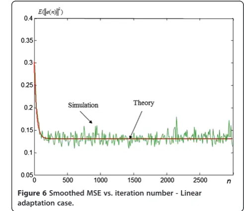
For the linear adaptation case (Section 3.1), the adaptive system is composed of a 2x2 matrix W. For the noise we have taken σ0 = 0.001. The mean weight recursions and

the MSE transient behaviors (Figures 6, 7) have been estimated over 20 Monte Carlo (MC) simulations and compared to the theoretical derivations (Equations (19) and (41)). This chosen number of MC simulations shows excellent fit between the Theory and MC estimations which confirms the validity of the different assumptions made. A larger number of MC simulations allows a bet-ter smoothing of the curves, but the conclusions remain the same.

Matrix W converges to a scaled version of H: W0¼

0:3536 0:0577 0:1061 0:1925

¼H U; U¼ 0:3536 0:0000

0:0000 0:1925

:

Note the typical behavior of the LMS algorithm: A time constant controls the transient part of the learning curve

(15)

and the mean weight curve. This is fundamentally differ-ent from the full NN system learning which is governed by several time constants and presents plateau regions (Section 5.2). It should be noted that the steady state MSE is high because of the error caused by the fact that the nonlinearities are not approximated (actually they are modeled by the identity function) (Equation (25)).

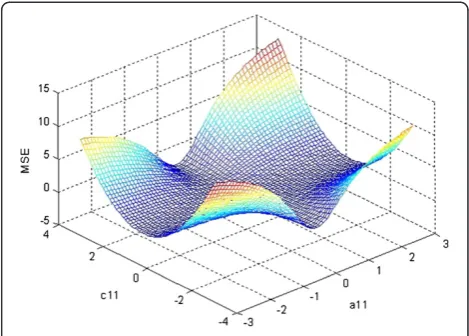
MSE surface for the full NN algorithm

We move now to the study of the full NN algorithm. In this simulation, we have taken N = 3 neurons in each of the two NN blocks. The learning rate was fixed toμ=0.0045. Figure 8 shows the MSE surface (i.e., Eq. (90), with no time dependence) as a function of w11

andw12(the other parameters were fixed). It is clear that

the MSE is quadratic inw11andw21. It presents a single

global minimum (as shown in Equations (76 and 84)).

Figure 9 (resp. Figure 10) shows the MSE surface as a function of a11 and c11 (resp. a11 and a12) (the other

parameters were fixed). It can be noted the flat areas (plateau regions) around the minima of the MSE sur-face. This explains the slow evolution of the NN weights when the algorithm gets close to its conver-gence point.

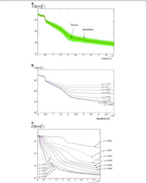
The MSE evolution during the learning process (Equa-tion (90)) has been compared to 20 MC estima(Equa-tions (Figure 11a): The theory shows very good fit with the simulation results. In the Figure, we notice that the MSE presents several phases (each phase is controlled by a time constant) which end by a plateau phase where the MSE decreases very slowly. This is a typical behavior of the backpropagation algorithm [1] which is fundamen-tally different from that of the linear adaptation scheme (Figure 6). Here the MSE error is much smaller. This is expected, since here the additional MSE error due to the nonlinearities (Eq. 92) is highly reduced because our NN

Figure 9MSE surface,MSE(a11,c21).

Figure 7Mean weight transient behavior - Linear adaptation case.

(16)

Figure 11a: MSE during the learning process (theory and simulation),σ0=0.001 andμ=0.0045. b: MSE for different values of noise variance, the learning rate wasμ=0.0045 (theoretical results).c: MSE for different values of learning rateμ(the noise variance was set toσ0=0.001),

(17)

blocks have correctly identified the unknown nonlineari-ties (Figure 12, 13). Here we are in a situation close to that of Section 3.2 (Equations 51-52).

Figure 11b shows the MSE evolution during the learn-ing process for different values of the noise varianceσ0.

It can be seen that, as the noise variance decreases, the MSE decreases. However, below a certain value of σ0

(here σ0=0.0005), the MSE curves are almost identical.

This is because in this case, the weight misadjustment error (for the linear part) and the nonlinear approxima-tion error (of the nonlinear memoryless part) are much higher than the error caused by the presence of noise (see Eqs. 92-93).

Figure 11c investigates the influence of the learning rateμ. It can be seen that asμincreases (up toμ=0.002), the algorithm is faster and the MSE is lower at the end

of the simulation time. However, for μ>0.002, as μ increases, the algorithm is faster at the beginning of the learning process, but the MSE is higher at the end of the simulation time. This is due to the misadjustment error which is higher for higherμ(see, e.g., Eq. 95).

Mean weight transient behavior for the full NN algorithm

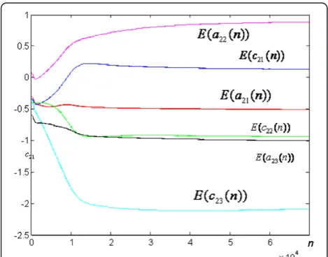
Here we keep the system described in Section 5.2. The mean weight recursions for the linear combiner W and the two NN blocks are shown in Figure 14, 15, 16 for both theory and MC estimations. The theoretical and estimated curves are indistinguishable. This confirms the validity of the different assumptions made in Sections 4.1 and 4.2.

Figure 12Identification ofg1(x), by the 1st_{NN block.}

Figure 13Identification ofg2(x) by the 2nd_{NN block.}

Figure 14Mean weight behavior: Matrix W (theory and simulation).

(18)

Notice that, in Figure 14, W weights have a fast evolution at the beginning of the learning process (with values approaching H×U(n) where U is a diag-onal matrix). They then evolve slowly till the end of the learning process. The slow evolution is justified by the plateau regions presented by the MSE surface. At the end of this simulation, matrix U was close to a diagonal matrix: USim¼ 1₀:_:2702₀₀₀₃ ₁0_::0001₀₉₄₆

; (and

UTheory¼ 1:270₀ ₁_:₀₉₅0

). This result is expected since the inputs are uncorrelated (Equations 84-85).

Figure 12, 13 show that functionsg1(x) andg2(x) have

been correctly identified by the corresponding NN blocks (the NN functions are normalized by the scaling factorsγ1=1/1.2702,γ1=1/1.0946, respectively).

Impact of correlated inputs

In the simulations below we study the impact of corre-lated inputs. The input signal vector is chosen here as a 2D Gaussian process with covariance matrix of the form

RXX ¼ 1_ρ ρ₁

: The number of neurons in each NN block was taken as N = 5 neurons. The learning rate

μ=0.0075. We have run several simulations for different

values of the cross correlation. Note that (ρ=0) corre-sponds to independent inputs, and (ρ=1) corresponds to the same input (i.e., x1=x2). The values of matrix U

and the MSE after n=2105 iterations are shown in Table 1. It can be seen from Table 1 that, in practice, matrix U remains very close to a diagonal matrix, even for high correlation between inputs. This indi-cates that the system is capable of correctly identifying the nonlinearities even when the inputs are highly correlated. The identification performances for the cases (ρ=0.6) and ( ρ=0.99) are illustrated in Figures 17, 18 and 19, 20, respectively. As expected, the MSE increases as the correlation between inputs increases (Table 1). When ρ=1 (i.e., the two inputs are the same) the system is capable of correctly identifying the overall MIMO input–output transfer function. However, in this case, it is not capable of separating the nonlinearities (as U is not diagonal). The reason is that in this case, the system is seen by the learning algorithm as a 1x2 SIMO system which has several equivalent structures. Figure 21 shows an example of two equivalent structures. There-fore, the adaptive system is structurally not able to separ-ate the nonlinearities. It is worth to note that for the case (ρ=0.999), the inputs look like noisy versions of each other (i.e., this is equivalent to a 1x2 system identifica-tion problem with noisy inputs). Thus, the MSE for the case (ρ=0.999 ) is larger than the MSE for the case (ρ=1).

Conclusion and future work

The paper provides a statistical analysis of NN model-ing and identification of a class of nonlinear MIMO systems. The study investigates the MSE error, mean weight behavior, stationary points, misadjustment error, and stability conditions. The unknown system is com-posed of a set of single-input memoryless nonlinearities followed by a combining matrix. The NN model is composed of a set of single-input memoryless NN blocks followed by an adaptive linear combiner. The paper is supported with simulation results which show good agreement between the theoretical recursions and MC simulations. Future work will focus on 3 research directions. The first will explore the theoretical findings in order to express the effect of the number of neu-rons on the transient and steady state behavior of the algorithm. The second research axis will investigate the Figure 16Mean weight behavior: Second NN block (theory and

simulation vs. iterations).

Table 1 Effect of correlated inputs

ρ=0 ρ=0.6 ρ=0.9 ρ=0.99 ρ=0.999 ρ=1 (same input)

E(U(n)), for

n=2 × 105 1:228 0:0000

0:0004 1:066

1_:2245 0_:0004

0:001 1:1331

1_:23 0_:001

0:0025 1:12

1_:24 0_:019

0:023 1:08

0_:324 1_:07 1:002 0:03

0_:023 1_:24 1:14 0:15

(19)

case where matrix H is time-varying and/or with mem-ory (this may have applications, for example, in adap-tive control of nonlinear dynamical MIMO systems). Finally, we will study the algorithm behavior and per-formance for specific inputs (such as space-time coded signals used in wireless communications and their im-pact on the system capacity).

Endnotes

This work has been supported by The Natural Sciences and Engineering Research Council of Canada (NSERC).

The time index of the weights has been omitted from the right hand side of the equations to make them easier to read.

Appendix I

1)Calculation ofFkk

Letx1andx2be two zero-mean Gaussian variables

such thatσ2

x1 ¼σ

2 x2¼σ

2

x and E xð 1x2Þ ¼ρ

Therefore,Fkkðaki;bki;akm;bkmÞ ¼E f akixð ð kð Þþn

bkiÞf akmxð kð Þ þn bkmÞÞ_ρ_¼_σ2

x:

Using Price’s theorem we have:

E @2f að kix1þbkiÞf aðkmx2þbkmÞ @x1@x2

h i

¼@E f a½ðkix1þbkiÞf wð kmx2þbkmÞ

@ρ :

LetUð Þ ¼ρ E @2f aðkix1þbkiÞf wð kmx2þbkmÞ @x1@x2

h i

;

Then:E f akix½ ð 1þbkiÞf akmxð 2þbkmÞ_ρ_¼_σ2

x

E f a½ ð kix1þbkiÞf að kmx2þbkmÞρ¼0¼ Rσ2

x

0 Uð Þρdρ:

Thus, using the un-correlation criteria betweenx1

andx2forρ=0 , we have:E f a½ ð kix1þbkiÞf að kmx2þ

bkmÞρ¼0¼E f a½ ð kix1þbkiÞE f a½ ð kmx2þbkmÞ:Thus:

Figure 17Identification ofg1(x), caseρ=0.6.

(20)

F að ki;bki;akm;bkmÞ ¼E f a½ ð kix1þbkiÞE f a½ ð kmx2þ

bkmÞ þRσ2x

0 Uð Þρ dρ:

We have:Uð Þ ¼ρ E @2f aðkix1þbkiÞf aðkmx2þbkmÞ @x1@x2

h i

¼

2

πakiakm₂_π1_{j j}_R1 2 Rþ1 1 Rþ1 1 e 1

2ðakix1þbkiÞ2_e12ðakmx2þbkmÞ2

e12XtR1Xdx₁dx₂ whereX¼½x₁x₂tand R¼ σ

2 x ρ

ρ σ2

x

:

Combining the terms in the exponentials and completing the squares, the integrals can be calculated:Uð Þ ¼ρ 2

π ffiffiffiffiffiffiffiffiffiffiffiffiffiffiffiffiffiffiffiffiffiffiffiffiffiffiffiffiffiffiffiffiffiffiffiffiffiffiffiffiffiffiffiffiffiffiffi₁_þ_σ2 akiakm

xa2kiþσ2xa2kmþðσx4 ρ2Þa2kia2km

p

exp 1₂ b2_kib2_kmþ 1

a2

kiþ σ2

x σ2

xρ2

"

b2_kia2_kiþ

" "

bkiaki a2kiþ σ2

x σ2

xρ2

þbkmakm_σ2ρ

xρ2

2 a2 kiþ σ2 x σ2

xρ2

a2 kmþ σ2 x σ2

xρ2

a2

km ρ

2

σ2

xρ2

3 5 3 5 3 5_:

Note that in the biasless case (i.e. all the bias terms are set to 0) this expression reduces to:

Uð Þ ¼ρ 2 π

akiakm

ffiffiffiffiffiffiffiffiffiffiffiffiffiffiffiffiffiffiffiffiffiffiffiffiffiffiffiffiffiffiffiffiffiffiffiffiffiffiffiffiffiffiffiffiffiffiffiffiffiffiffiffiffiffiffiffiffiffiffiffiffiffiffiffiffiffiffiffiffiffiffiffiffi

1þσ2

xa2kiþσ2xa2kmþ σ4xρ2

a2

kia2km

q :

The integral is then simple to calculate:

Z σ2

x

0

Uð Þρ dρ¼2 πsin1

akiakmσ2x

ffiffiffiffiffiffiffiffiffiffiffiffiffiffiffiffiffiffiffiffiffiffiffiffiffiffiffiffiffiffiffiffiffiffiffiffiffiffiffiffiffiffiffiffiffiffiffiffiffiffiffiffiffi

1þσ2

xa2kiþσ2xakm2 þσ4xa2kia2km

q 0 B @ 1 C A

In the other hand, sinceE f w½ ð kx1Þ ¼E f w½ ð ix2Þ ¼0,

then:

F að ki;akm;0;0Þ ¼2_πsin1 akiakmσ 2

x

ffiffiffiffiffiffiffiffiffiffiffiffiffiffiffiffiffiffiffiffiffiffiffiffiffiffiffiffiffiffiffiffiffiffiffiffiffiffi 1þσ2

xa2kiþσ2xakm2 þσ4xa2kia2km p

:

When the bias terms are not set to 0, a Taylor series expansion on the bias terms can be used in order to avoid the calculation of the integral.

2) Calculation ofK

Kkðakm;bkmÞ ¼E g½kð Þxk f akmxð kþakmÞ

¼ 1ffiffiffiffiffiffi

2π

p _σ1

x Z þ1

1 αkx e βk x22_e

x2

2σ2

x

Z akmxþbkm

0

eu 2 2_{du dx}:

The inside integral can be eliminated by integrating

by parts on variablex.

The integral is then evaluated by combining the terms in the exponentials and completing the squares. This yields:

Kkðakm;bkmÞ ¼ ffiffiffi 2 π r αk 1 σ2

xþβk

akm

ffiffiffiffiffiffiffiffiffiffiffiffiffiffiffiffiffiffiffiffiffiffiffiffiffiffiffiffiffiffiffiffiffiffiffi

σ2

x a2kmþβk

þ1

q

exp b

2

km

2 1

σ2 x

1þσ2

x βkþa2km

!! :

Again, a Taylor series expansion can be used to simplify this expression.

Note that in the biasless case we have:

Kkðakm;0Þ ¼

ffiffiffi 2 π r α 1 σ2

xþβk

akm

ffiffiffiffiffiffiffiffiffiffiffiffiffiffiffiffiffiffiffiffiffiffiffiffiffiffiffiffiffiffiffiffiffiffiffi

σ2

x a2kmþβk

þ1

(21)

Appendix II

The derivatives needed to compute the different recursions are expressed as follows:

@Kkðakm;0Þ @akm ¼

ffiffiffi 2 π r ασ2 x σ2

x a2kmþβk

þ1

3

2;

@Kkðakm;bkmÞ @akm ¼

@Kkðakm;0Þ @akm

ffiffiffi 2

π

r

αk σ2x

b2

km 2

1þσ2

xβk2σ2xa2km 1þσ2

x βkþa2km

5

2 @Fkkðaki;0;aki;0Þ

@aki ¼ 4

π

σ2

xaki

σ2

xa2kiþ1

ffiffiffiffiffiffiffiffiffiffiffiffiffiffiffiffiffiffiffiffiffiffi 1þ2σ2

xa2ki

q ;

@Fkkðaki;aki;bki;bkiÞ

@aki ¼

@F að ki;0;aki;0Þ

@aki

2

πb2kiσ2xaki

5σ2_xa2_kiþ3 1þσ2

xa2ki

2

1þ2σ2

xa2ki

3

2 @F að ki;0;akm;0Þ

@aki ¼ 2

π

σ2

xakm

σ2

xa2kiþ1

x a2kiþa2km

q

@F að ki;akm;bki;bkmÞ

@aki ¼

@F að ki;aki;0;0Þ

@aki

1

πb2ki

σ2

xakm

1þσ2

xa2ki

x a2kmþa2ki

q 1þσ2xa2km

1þσ2

x a2kmþa2ki

2σ2xa2ki 1þσ2

xa2ki !

_π1a2_km σ

2

xakm 1þσ2

x a2kmþa2ki

3

2 bkibkm

2

π

σ2

xaki 1þσ2

x a2kmþa2ki

3

2 @F að ki;akm;bki;bkmÞ

@bkm ¼

2

πbki σ

2

xakiakm

1þσ2

xa2ki

x a2kmþa2ki

q bkm

2

π

1

x a2kmþa2ki

q

Appendix III

2μKVjVjð ÞRn XX

þ2μE eW0jð Þn XV

t

jðI2μXXtÞ

h i

þ2μE eW0jð ÞXVn

t

jðI2μXXtÞ

h it

þ4μ2E XXtKVjVjXX t

þ4μ2E e2_W₀_jð ÞXXn t

h i

ð96Þ The calculations are similar to [9] Appendix, the main difference is that here we deal with a multi-dimensional input. Therefore, we will follow the same methodology as in [9].

Following [10] the expectation before the last one can be calculated as:

E XXtKVjVjð ÞnXX t

¼tr RXXKVjVjð Þn

RXX

þ2RXXKVjVjð ÞRn XX: ð97Þ

The first expectation is expressed as:

E eW0jð ÞXVn t

jðIμXXtÞ

h i

¼E eW0jð ÞnXV t j

h i

μE eW0jð ÞnXV t jXXt

h i

ð98Þ

The first term is Zero (orthogonality principle). The second term is:

E eW0jð ÞnXV t jXXt

h i

¼E H_jtgj xj þNjð Þn

h

Wt

0jX nð Þ

XV_jtXXt

i

ð99Þ

The middle term is Zero (Zero-mean white noise), the last expectation is:

E W₀t_jX nð ÞXV_jtXXt

h i

¼E X nð ÞXW0Vjtð Þn XXt

h i

tr RXXW0E Vjtð Þn

RXX

þ2RXXW0E Vjtð Þn

RXX

ð100Þ

The first expectation in Eq. (99)E Ht

jg Xð ÞXVjtð ÞXXn t

h i

E Ht

jg Xð ÞXE Vjtð Þn

XXt

h i

involves the nonlinearity gj

(xj) and should be evaluated explicitly. The remaining expectation in (96) is:E e2

ojð ÞnXXt

h i

:

E eh 2_ojð ÞnXXti¼E H_jtg Xð Þ W₀t_jX2XXt

þσ2 0RXX

(22)

We have

E W₀t_jX2XXt

¼E XXh tW₀t_jW₀t_jXXti

¼tr RXXW0tjW0tj

RXX

þ2RXXW0tjW t

0jRXX ð102Þ

The first term in (102) is:

E H_jtg Xð Þ2XXt

¼E HjHjtg Xð Þg t_{ð Þ}_X _XXt

h i

¼E g Xð Þgtð ÞX HjHjtXX t

h i

(96) is then expressed as:

2μKVjVjð ÞnRXXþ4μ

2 _{E H}t

jg Xð ÞXE Vjtð Þn

XXt

h i

RXXþRXXW0E Vjtð Þn

RXX

XXt

h i

RXXþRXXW0E Vjtð Þn

RXX t

þ4μ2 tr RXXKVjVjð Þn

RXX þ2RXXKVjVjð ÞRn XX

þ4μ2 E g Xð Þgtð ÞHX jHjtXXt

h i

þσ2 0RXX

tr RXXW0tW0t

RXX2RXXW0tjW0tjRXX

Competing interests

The author declares that he has no competing interests.

Received: 6 December 2011 Accepted: 13 July 2012 Published: 21 August 2012

References

1. S. Haykin,Neural Networks: A Comprehensive Foundation(Prentice Hall, 1999) 2. Y. Gao, M. Er, Online adaptive fuzzy neural identification and control of a

class of MIMO nonlinear systems. IEEE Trans. Fuzzy Systems, 462_–476 (2003) 3. S.S. Ge, C. Wang, Adaptive neural control of uncertain nonlinear MIMO

systems. IEEE Trans. Neural Networks15, 674_–692 (2004)

4. M. Ibnkahla, A. Al-Hinai, Adaptive modeling and identification of nonlinear MIMO channels using neural networks, inAdaptive Signal Processing in Wireless Communications, ed. by M. Ibnkahla (CRC Press, Boca Raton, FL, USA, 2008)

5. K.S. Narendra, K. Parthasarathy, Identification and control of dynamical systems using neural networks. IEEE Trans. Neural Networks1, 4–27 (1990) 6. H. Xu, P. Ioannou, Robust adaptive control for a class of MIMO nonlinear

systems with guaranteed error bounds. IEEE Trans. Automatic Control, 718_–742 (2003)

7. S. Amari, Mathematical foundations of neurocomputing. Proc. IEEE 78(9), 1443–1463 (September 1990)

8. N.J. Bershad, M. Ibnkahla, F. Castanié, Statistical analysis of a two-layer back propagation algorithm used for modeling non linear memoryless channels: The single neuron case. IEEE Trans. Signal Processing45(3), 747_–756 (March 1997)

9. N. Bershad, P. Celka, J.M. Vesin, Stochastic analysis of gradient adaptive identification of nonlinear systems with memory for Gaussian data and noisy input and output measurements. IEEE Trans. Signal Processing 47(3), 675–689 (March 1999)

10. S. Haykin,Adaptive Filter Theory(Prentice Hall, 1996)

11. M. Ibnkahla, N.J. Bershad, J. Sombrin, F. Castanié, Neural network modeling and identification of non linear channels with memory: Algorithms, applications and analytic models. IEEE Trans. Signal Processing46, 5 (1998) 12. M. Ibnkahla, Statistical analysis of neural network modeling and

identification of nonlinear channels with memory. IEEE Trans. Signal Processing, 1508_–1517 (2002)

13. J. Shynk, S. Roy, Convergence properties and stationary points of a perceptron learning algorithm. Proc. IEEE70, 1599_–1604 (Oct. 1990) 14. J.G. Taylor,Mathematical Approaches to Neural Networks(North-Holland,

Amsterdam, 1993)

15. H. White, learning in artificial neural networks: A statistical perspective. Neural Comput.1, 425–464 (1989)

16. N. Bershad, P. Celka, J.M. Vesin, Analysis of stochastic gradient tracking of time-varying polynomial Wiener systems. IEEE Trans. Signal Processing 48(6), 1676_–1686 (June 2000)

17. H. Bolcskei, MIMO systems: Principles and trends, inSignal Processing for. Mobile Communications Handbook, ed. by M. Ibnkahla, 12th edn. (CRC Press, 2004)

18. T. Javornik, G. Kandus, S. Plevel, G. White, A. Burr, V-BLAST algorithm performance in non-linear channel. IEEE Computer as a Tool Conference 1, 183–187 (September 2003)

19. G. Poitau, A. Kouki, Impact of realistic amplification models on dynamic VBLAST optimization. Proc. Vehicular Technology Conference Spring, 894_–897 (2004)

20. S. Woo, D. Lee, K. Kim, H. Hur, C. Lee, J. Laskar, Combined effects of RF impairments in the future IEEE 802.11n WLAN systems. Proc. IEEE Vehicular Technology Conference Spring2, 1346–1349 (May 2005)

21. S. Yang, J. Xi, X. Mu, Decision aided joint compensation of clipping noise and nonlinearity for MIMO-OFDM systems. Proc. IEEE International Symposium on Communications and Information Technology (ISCIT) 1, 725–728 (2005)

22. S. Yang, J. Xi, F. Wang, X. Mu, H. Kobayashi, Decision aided compensation of residual frequency offset for MIMO-OFDM systems with nonlinear channel. Proc. International Symposium on Intelligent Signal Processing and Communication Systems (ISPACS), 113_–116 (2005)

23. A. Sulyman, M. Ibnkahla, Performance of MIMO systems with antenna selection over nonlinear fading channels. IEEE Journal in Selected Topics in Signal Processing2, 159–170 (April 2008)

24. A. Sulyman, M. Ibnkahla, Performance analysis of nonlinearly amplified M-QAM signals in MIMO channels. European Transactions in Communications 19(1), 15–22 (January 2008)

25. J. Pedro, S. Maas, A comparative overview of microwave and wireless power amplifier behavioral modeling approaches. IEEE Trans. Microwave Theory and Techniques53(4), 1150_–1163 (2005)

26. A. Saleh, Frequency-independent and frequency–dependent nonlinear models of TWT amplifiers. IEEE Trans. Communications29, 11 (1981)

doi:10.1186/1687-6180-2012-179

Cite this article as:Ibnkahla:Stochastic analysis of neural network modeling and identification of nonlinear memoryless MIMO systems.

EURASIP Journal on Advances in Signal Processing20122012:179.