Molecular dynamics investigation of carbon nanotube junctions in non aqueoussolutions

Molecular dynamics investigation of carbon

nanotube junctions in non-aqueous solutions

K. Gkionis,aJ. T. Obodo,aC. Cucinotta,bS. Sanvitoband U. Schwingenschl¨ogl*a

The properties of liquids in a confined environment are known to differ from those in the bulk. Extending this knowledge to geometries defined by two metallic layers in contact with the ends of a carbon nanotube is important for describing a large class of nanodevices that operate in non-aqueous environments. Here we report a series of classical molecular dynamics simulations for gold-electrode junctions in acetone, cyclohexane andN,N-dimethylformamide solutions and analyze the structure and the dynamics of the solvents in different regions of the nanojunction. The presence of the nanotube has little effect on the ordering of the solvents along its axis, while in the transversal direction deviations are observed. Importantly, the orientational dynamics of the solvents at the electrode–nanotube interface differ dramatically from that found when only the electrodes are present.

Introduction

Nanoscale devices have attracted intense interest among researchers over the past decades, due to their wide range of applications. Biotechnology is an example of a eld where advances in nanotechnology can be highly benecial. Applica-tions range from drug delivery1and DNA sequencing2to tissue engineering3 _{and sensing devices.}4,5 _{The latter technological} area oen employs carbon nanotubes (CNTs) as active element for the detection of the species of interest. In fact, single or multi-walled nanotubeeld-effect transistors are oen used in biosensors, in which the nanotube is mounted between elec-trodes and the analyte is detected by its effect on the electrical response of the CNT itself.

Since species of biological interest typically appear in an aqueous environment, biosensors are aimed at functioning in wet conditions, although devices functioning in non-aqueous solutions are also of interest. For example, Gr¨uner and co-workers have investigated the interactions of different benzene derivatives with CNTs in non-aqueous media, such as cyclo-hexane, revealing a linear relationship between the gate voltage shis and the Hammett constants of the benzene substituents.6 The same study has compared theI–Vcharacteristics of the CNT eld-effect transistors immersed in non-aqueous media and in air. Along the same lines, the dependence of the response on the size of the aromatic compounds and the detection of amine derivatives has been investigated,7_{both being of interest in the} context of hydrocarbon fuels.

The presence of a medium, whether aqueous or non-aqueous, affects the electrical response of a device and thus has to be taken into account in a measurement. The electrodes of a sensor act as conning walls for the solvents, which in turn exhibit different properties than those in the absence of connement. Hence, knowledge of the behavior of conned solvents in the presence of CNTs in a typical device geometry is important for understanding the function of the device itself. Spectroscopy can be used for investigating the orientations of solvents and molecules in metal–CNT junctions. Specically, the orientation of the molecules has been addressed by Raman spectroscopy and the orientational dynamics have been explored by second harmonic generation measurements.8,9 Nowadays sufficiently long molecular dynamics (MD) simula-tions of large systems are feasible to complement such experi-ments by providing details at the molecular level.

In general, computational modeling is a valuable tool for studying material properties. For example, MD simulations are routinely employed to investigate structural and dynamical aspects of conned liquids10,11 _{and nanotubes in wet} condi-tions.12 _{Similarly,ab initio calculations provide the electronic} structure of matter and are useful in predicting transport prop-erties in nanojunctions. Importantly, a combination of MD and

ab initiocalculations allows one to evaluate the transport prop-erties of nano-devices in wet conditions, by taking into account the dynamical behavior of the solvents in an averaged manner.13 Although various MD studies of conned liquids and nano-tubes have been reported in the literature, to the best of our knowledge work on nanojunctions in solution is still lacking. Previously, the Gao, Luedtke and Landman approach14has been employed for the study of conned liquids and it has been demonstrated that such a setup is useful for analyzing nano-tube–electrode nanojunctions.15_{In particular, the efficiency of}

a_{KAUST, PSE Division, Thuwal 23955-6900, Kingdom of Saudi Arabia. E-mail: udo.}

schwingenschlogl@kaust.edu.sa; Tel: +966 544700080

b_{School of Physics and CRANN, Trinity College, Dublin 2, Ireland} Cite this:J. Mater. Chem. A, 2014,2,

16498

Received 1st June 2014 Accepted 23rd July 2014

DOI: 10.1039/c4ta02760d

www.rsc.org/MaterialsA

Materials Chemistry A

PAPER

Published on 23 July 2014. Downloaded by Trinity College Dublin on 28/01/2015 12:07:58.

the procedure for estimating the number of molecules within the junction in the presence of a nanotube has been stressed. In the present study we employ the same approach to investigate the structure and the dynamics of non-aqueous solvents, namely acetone, cyclohexane and N,N-dimethylformamide (DMF) in Au/CNT/Au junctions. Note that all the three solvents are of potential interest in theeld of hydrocarbon fuels.6,7

Methods

Fig. 1 displays the three solvent molecules considered in this study, namely acetone, cyclohexane and DMF, while the geometry of the device investigated, along with the reference Cartesian axes, is shown in Fig. 2. This geometry is convenient for our device setup.15In fact the presence of the nanotubexes the distance between the two electrodes and therefore the size of the cell in the

direction of the nanotube, so that a barostat-type optimization is impossible. We use electrodes with periodic boundary conditions in thex-direction only to reduce the complexity of adjusting the solvent's density for a given pressure by varying the volume.15_We now investigate the structure and the dynamics of Au/CNT/Au nanojunctions immersed in different liquid solvents. In partic-ular the properties of the nanoconned solvents are compared to those obtained under the simple connement provided by two Au electrodes only,i.e., in the absence of the nanotube. The aniso-tropic arrangement of the nanotube in our model enables us to gain insight into the effect of different connement geometries on the behavior of the solvents.

The electrodes expose their Au(111) surfaces and have dimensions of 1.63.90.9 nm3, consisting of 5 layers of gold with 96 atoms per layer. This results in a total of 960 gold atoms. The CNT is 3.7 nm long, it has a diameter of 0.6 nm, and comprises 288 carbon atoms. The distance between the CNT and each of the electrodes is keptxed at 0.21 nm (a value obtained withab initiooptimization16_{). Thus the surfaces of the electrodes} are separated by 4.15 nm. The solvent molecules partially surround the electrodes, as shown in Fig. 2, thus only a portion of the solvent is conned between the electrodes and the molecules are also in contact with the electrodes' sides. The number of solvent molecules used in our simulations is respectively 600 for acetone, 300 for cyclohexane and 500 for DMF. Moreover, the simulation box in thexz-plane spans an area of 1.76.3 nm2in all cases, with they-dimension being readjusted by means of an isobaric simulation (see below for further details). The dynamics of the structural morphology are studied at zero bias. Finite bias might slightly affect the alignment (polarization) of the mole-cules of the solvent and thus the electrical response.

All calculations are performed with the NAMD soware17and the implemented CHARMM force-eld.18CHARMM parameters are employed for the description of cyclohexane and the aromatic carbon atoms of the CNT, while for DMF and acetone we use the CHARMM General Force Field parameterization.19 Finally, gold is described by the parameterization of Heinz and co-workers.20_{Gold and CNT atoms are neutral and keptxed at} their ideal positions during all the simulations. Bonds involving hydrogen atoms are kept rigid for all the solvents and the cyclohexane is kept rigid in its most stable chair conformation. Non-bonding interactions between heteroatoms are described by the Lorentz and Berthelot mixing rules,i.e., by employing the arithmetic mean for the contact distance, rmin,ij, and the geometric mean for the interaction energy,3ij, of the Lennard-Jones potential. For atoms separated by more than 1.0 nm they smoothly vanish beyond 1.2 nm. For interatomic distances larger than this threshold the non-bonding interactions are included as a correction.21Long-range Coulomb interactions are described by using the particle-mesh Ewald method22_{for computing the Ewald} summation.23_{Electrostatic interactions are evaluated every 4 fs,} while the timestep of the simulation is 2 fs.

All systems are initially treated by energy minimization for 5000 steps in order to eliminate steric clashes. Subsequently, the systems are gradually heated to the target temperature of 300 K at a rate of 0.5 K every 200 fs by using the velocity reas-signment method. Aer these initial steps all the systems are Fig. 1 The three solvents considered in this work: from left to right:

acetone, cyclohexane and DMF.

Fig. 2 The geometry of the devices simulated and the reference Cartesian axes. Au atoms are shown as yellow spheres, C atoms as grey capped sticks.

simulated in the isothermal–isobaric ensemble (NPT) at 1 atm for 160 ns, during which thexzarea is kept constant and only the y-dimension is allowed to readjust. The pressure is kept constant by the Nos´e–Hoover method24and the piston uctua-tion control25with a piston period of 400 fs, decay of 200 fs and temperature of 300 K. The equilibrium size of every cell along they-direction is obtained by averaging out the values of the NPT simulation (see Table 1). This scheme for optimizing the cell volume allows us to control the density of the system.

Subsequently, a NVT simulation is performed for 2 ns with the volume dened by the initial x- and z-dimensions (kept constant) and the averagey-dimensions listed in Table 1. For both the NPT and NVT simulations the temperature is controlled by a local Langevin thermostat with a Langevin coefficient of 5 ps1_{applied to all atoms. Once the systems are} equilibrated the thermostat is removed and the microcanonical ensemble (NVE) is employed for 2 ns, during which the trajec-tory is recorded every 10 fs for analysis.

Results

Fig. 3 displays the obtained proles along thez-axis for the region in which the solvent molecules are conned between the gold electrodes. An advantage of our model is that the two surfaces of the metal electrodes are equivalent, thus that the density proles are symmetric with respect to the median plane of the device. As a consequence we can average over two half cells, decreasing the statistical error in the computation of the density proles.

In all cases we obtain typical proles of conned liquids, with peaks of higher density next to the gold surfaces, which gradu-ally disappear away from the surface. An exception is the case of cyclohexane, which exhibits a more structured density prole along thez-axis, as predicted before.26,27The density peaks due to the proximity to the surfaces occur at distances of 3.3˚A for all solvents and irrespective of whether or not the CNT is present. For acetone and DMF a second peak appears respectively at 7.0 and 6.6˚A from the surface, andnally near the middle of the junction (beyond 17A in Fig. 3) the density eventually tends to a˚ constant value. In this region the average densities of acetone, cyclohexane and DMF are 0.809 g cm3 (0.03), 0.740 g cm3 (0.32) and 0.994 g cm3(0.04), respectively (in brackets we report the standard deviations). These values are very close to the reported values28_{of 0.791, 0.779 and 0.944 g cm}3_{. Cyclohexane} in this region exhibits the mentioned oscillations, ranging from 0.330 to 1.199 g cm3both when the CNT is present or not.

In the same region the density of a solvent in the presence of the CNT averages to a lower value than that obtained in the absence of the CNT, namely 0.721, 0.665 and 0.876 g cm3for acetone, cyclohexane and DMF, respectively. This behavior is due to the volume occupied by the nanotube and it is not an indi-cation that the actual density drops. In fact the ratios of the average densities calculated either without and with nanotubes for each solvent are almost identical (acetone: 1.12, DMF: 1.13, cyclohexane: 1.11). The volume of the CNT is the same in all cases and the minor discrepancies observed are attributed to subtle differences among the solvents, related to the additional volume excluded by the nanotube–solvent non-bonding interactions.

We further evaluate the density proles along the y-axis (Fig. 4, le). In this case, we consider a slab that is only 5˚A thick along thez-direction (blue lines labeled as“middle”in Fig. 4). The slab is taken in the central region of the junction in order to maintain the distance to each surface as large as possible (approximately 18A). As expected, in the absence of the CNT the˚ densities for this region remain practically constant, as if there was only a bulk solvent (blue dashed line in Fig. 4). We obtain 0.802 (0.01), 0.780 (0.04) and 0.982 (0.04) g cm3for acetone, cyclohexane and DMF, respectively. The presence of the CNT perturbs the proles and peaks are obtained near the CNT, indicating that the solvents assume structures similar to solvation layers. In all the cases the density is increased at a distance ranging between 3.3˚A and 3.4˚A from the CNT, in a rather similar way to therst peak observed for the gold surface. A second, although rather small, peak is observed at larger distances (8˚A to 9A) from the CNT for all the solvents,˚ i.e., at a signicantly larger distance than the second peaks computed for Au.

Table 1 Average length of the systems in they-direction after NPT equilibration

System y(nm)

Acetone 7.9 Acetone, CNT 8.2 Cyclohexane 6.2 Cyclohexane, CNT 6.5

DMF 7.1

DMF, CNT 7.4

Fig. 3 Density profiles along thez-axis for the entire system. Hori-zontal blue dashed lines represent the calculated average density in the bulk. The Au surface boundary is atx¼0.

In order to study the extent of the perturbation introduced to the density proles by thenite nature of the electrodes along they-axis (the edge is represented by the red line in Fig. 4), we plot the density prole along this direction considering the entire system (black lines in Fig. 4, le). While the general trend of the prole is reproduced, in the conned region the density plots are shied to lower values. This is a direct effect arising from the larger volume. It is interesting to note that in the region within the electrodes (between the green and red dashed lines in Fig. 4) the average density is not strongly affected by the presence of the electrode edge. Instead, the edge perturbs the proles in the region between 20A and 25˚ A in Fig. 4,˚ i.e.outside the conned region, where a peak is observed in all proles. These peaks are similar to those observed near the Au(111) surface (see Fig. 3), but here they are due to the proximity of the solvents to the side of the electrode. In all cases, beyond this perturbation (distances longer than 25A) all pro˚ les converge to approximately the same value. An exception is cyclohexane, for which all proles are noisy and maintain averages between 0770 g cm3and 0.815 g cm3.

Another point of interest is the average density prole along they-direction, measured over a slice that is adjacent to the surface. We consider a 5A-thick slice so that to roughly corre-˚ spond to the solvent molecules that are enclosed within therst density peak along thez-axis (Fig. 3). In this case, the density of thisrst layer of solvent molecules next to the surface oscillates both when a CNT is present and when it is absent. The main difference between the two cases is the reduced density in the region occupied by the CNT. The oscillations are the result of the fact that the slice contains only the molecules adjacent (adsorbed) to the surface. Thus, the prole is largely affected by the intramolecular atomic arrangement of each solvent.

A third prole is evaluated for two equal-sized regions around the CNT, as schematically displayed in Fig. 5. These two

proles, presented in Fig. 6, are evaluated in order to determine the effect of different connement geometries along thex-axis, since in our systems the periodic images of the CNT in the

x-direction are much closer than those along they-direction. Fig. 4 Left: the density profiles along they-axis for the entire system (all) and for a slice cut in the middle of the junction (middle). Right: density profiles along they-axis at the electrode surface. In all the graphs continuous and dashed lines correspond respectively to the presence and the absence of the CNT. Vertical dashed green and red lines indicate the boundary along they-axis of the CNT and the electrode, respectively.

Fig. 5 Top view of the Au/CNT/Au device investigated. The blue rectangles on the left-hand side indicate the spatial regions around the CNT (ring) used to construct the density profiles reported in Fig. 6. The black rectangle on the right-hand side highlights the periodic image along thex-direction.

The peaks in the proles due to the CNT connement effect are found at the same position for both directions. However, a notable difference in the magnitude of the peaks is observed. In the cases of acetone and DMF the peak is more pronounced along the x-direction, due to the proximity of the periodic images, which acts as additional connement and enhances the ordering of the solvents. However, this feature is not observed for cyclohexane, where the peaks along thex- andy-directions are practically identical. Such a difference is probably due to the lessexible geometry of cyclohexane as compared to acetone and DMF, which prevents a stronger ordering than that already induced for this system geometry.

While the density proles examined above reect the ordering due to the connement, the formalism of the second order parameter can provide additional insights into whether there are deviations from a random arrangement of the mole-cules at or near the interfaces. The second order parameter is given by:

P2 cosq¼3₂cos2_ðqÞ 1

2 (1)

where q is the angle between an arbitrary vector along the solvent molecule and thez-axis. The squared cosine is averaged over 2500 snapshots of the trajectories. The molecular vectors are oriented along the C]O bond for acetone, along the bond between the C atom in the carbonyl group and N for DMF and along two opposite C atoms (all C atoms are equivalent) for cyclohexane. The possible most interesting values of P2 are 0.5, 1.0 and 0.0, which correspond to perpendicular, parallel and random orientation of the molecular vector with respect to thez-axis, respectively.

Fig. 7 shows the order parameter calculated by considering the trajectories only of molecules positioned within the conned region,i.e. those in between the two Au electrodes. Similar to the respective density prole along the z-axis, the pattern of the order parameter is maintained whether the CNT is present or not, for acetone and DMF, while cyclohexane does not follow the same trend. In all six curves of Fig. 7,P2attains negative values near the surfaces, with the most negative values for the adsorbed solvents on the surface, i.e., the layer that corresponds to the density peaks. This indicates a tendency to an orientation parallel to the Au surface, which is more pronounced for DMF and cyclohexane.

The area where the angular orientation deviates from randomness roughly corresponds to therst minimum of the density along thez-axis (see Fig. 3). In cyclohexane this area tends to be larger and the onset of randomness is more gradual, which can be explained on the basis of the adopted orientations per layer. A snapshot of the cyclohexane system is shown in Fig. 8, where it is evident that molecules next to the surface have Fig. 6 Density profiles calculated for two narrow regions cut around

the CNT respectively along the x- and y-direction (top: acetone, middle: cyclohexane, bottom: DMF). Thex¼0 position corresponds to the boundary of the nanotube. The regions used for the calculations are shown in Fig. 5.

Fig. 7 Order parameter profile along the z-axis for molecules included in the confining region.

Fig. 8 Spatial distribution of cyclohexane molecules (shown as green planar chains for clarity) near the Au surface. Note that order is progressively lost as one moves away from the surface.

a clear tendency to orient themselves parallel to the surface. Molecules in the second layer from the surface still exhibit this tendency, although much weaker. The onset of randomness in the second layer and beyond is gradual.

Away from the surface and near the middle of the deviceP2 becomes practically zero, indicating a random orientation of the solvent molecules. This is consistent with the observation that the average density resembles that of the unconned solvent, while for cyclohexane minor oscillations of the order parameter are observed, reecting the oscillatory behavior of the density.

Additional insights into the effects arising from the Au surface and the CNT on the solvent are gained by plottingP2 against they-axis for molecules that are found in the middle between the surfaces (conned region) or adjacent to each surface (Fig. 9). In thisgure the full lines correspond to the device incorporating the CNT, while the dashed lines are for the two Au electrodes only. The values along the horizontal axis denote the distance from the central axis of the CNT (y¼0). Similar patterns are obtained for all the solvents when consid-ering the molecules adjacent to the Au surface, whether the CNT is present or not. The order parameterP2maintains a negative value up to approximately 22˚A away from the center of the CNT, where it then grows to almost or even above zero for additional 3–4A and˚ nally converges to zero (beyond 25˚A). The region whereP2is close to zero corresponds to the volume beyond the boundaries of the electrodes, where a random orientation of the molecules is to be expected. This fact is consistent with the density prole along they-axis, see Fig. 4, where we obtain bulk values in this same region. In the conned region (below 20˚A) the order parameters are constantly negative, ranging from

0.2 for acetone to0.45 for cyclohexane and DMF, as expected by the prole along the z-axis (Fig. 7). The slightly positive values in the region between 20 A and 25˚ ˚A are due to the

molecules that lie on the yz-sides of the electrodes. In this region density peaks are observed along the same direction. Hence, such an effect is absent when only the middle region is considered (blue lines). In this caseP2is nearly zero all along they-axis, indicating that away from the surfaces all solvents orient themselves randomly, consistent with the fact that the densities approach bulk values. Since the interaction between the CNT and solvent does hardly depend on the surface curva-ture, the above results are expected to apply also to CNTs of larger diameter.

Fig. 9 Second order parameterP2(cos(q)) profiles along they-axis for molecules in the middle between the surfaces (middle) and for molecules adjacent to the surfaces (surface). Continuous lines corre-spond to the presence of the CNT, dashed lines to its absence. Vertical green and red dashed lines indicate the boundaries of the CNT and Au surface, respectively.

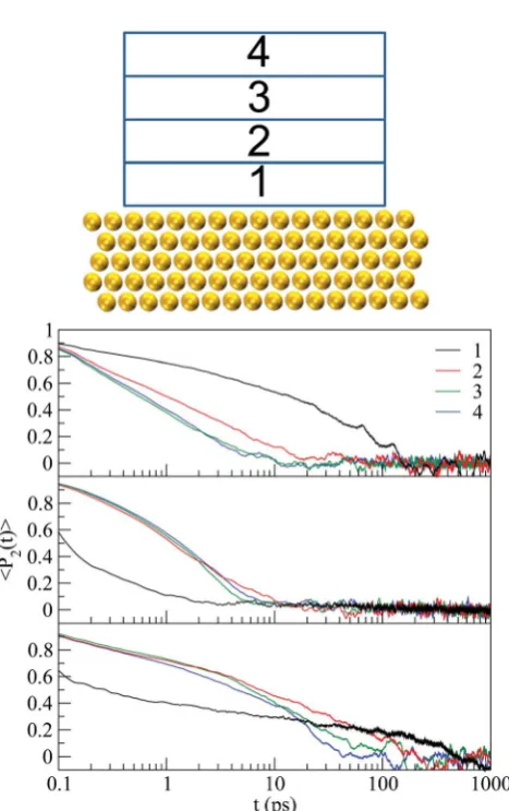
Fig. 10 Autocorrelation function for the order parameterP2(t) as a function of time: device not incorporating the CNT. From top to bottom we present results for acetone, cyclohexane and DMF. The numbers label the regions used in the calculation, which are displayed in the top panel.

Both the density proles and the order parameter analyzed so far provide useful information on the system ordering, but no insight into its dynamics. Thus, we next focus on the orientation dynamics of the solvent molecules as a function of their distance from the surface and from the nanotube. To this aim, we consider the autocorrelation times <P2(t)> of the order parameter. The molecular vectors for the three solvents are those dened before when calculatingP2(cosq). A plot of the investigated region and the corresponding autocorrelation diagrams are displayed in Fig. 10–12. The actual regions

considered have been chosen to correspond to each solvent's density prole. We expect that the autocorrelation times for the system without the CNT (Fig. 10) and far away from the CNT (Fig. 12) are similar. In particular, longer autocorrelation times should be observed for region 1 (see Fig. 10–12), as it has been shown for the case of benzene conned between Au(111) surfaces.11

Longer autocorrelation times for region 1 are evident for all solvents (around 150–200 ps, 100 ps and 400–500 ps for acetone, cyclohexane and DMF, respectively) when no CNT is present (Fig. 10). For acetone and cyclohexane wend similar trends in Fig. 12, as expected, although longer autocorrelation times are Fig. 11 Autocorrelation function for the order parameterP2(t) as a

function of time: device incorporating the CNT and measurement regions close to the CNT. From top to bottom we present results for acetone, cyclohexane and DMF. The numbers label the regions used in the calculation, which are displayed in the top panel.

Fig. 12 Autocorrelation function for the order parameterP2(t) as a function of time: device incorporating the CNT and measurement regions far from the CNT. From top to bottom we present results for acetone, cyclohexane and DMF. The number labels the regions used in the calculation, which are displayed in the top panel.

observed (around 100 ps). This is due to the fact that the volume of region 1 in Fig. 12 is smaller than that in Fig. 10. The respective region next to the CNT (Fig. 11) yields signicantly longer autocorrelation times for cyclohexane (above 600 ps) and slightly longer for acetone (above 300 ps), since the molecules in region 1 adjacent to the nanotube are under the inuence of the Au surface as well as the CNT, resulting in a slower reor-ientation. For DMF the correspondence between Fig. 10 and 12 is not as evident: in the latter case the curve seems to reach zero more rapidly than when the CNT is absent, a trend opposite to that for acetone and cyclohexane. However, it must be noted that while in most cases the curves oscillate around zero at long times, in Fig. 12 the negative values are more pronounced. Taking this negative correlation into account the de-correlation time is close to 1 ns, consistent with the increase observed for the other two solvents. On the other hand, shorter autocorre-lation times are observed for DMF in the respective region next to the CNT (Fig. 11), in contrast to acetone and cyclohexane.

Concerning layers 2 to 4, no clear trend is observed. There is a tendency for layer 2 to yield longer autocorrelation times than layers 3 and 4 when the CNT is absent (Fig. 10) for all solvents, while this situation becomes more complex with the CNT. This behavior is connected with the observed density proles for acetone and cyclohexane, which show that beyond the second peak any structure practically disappears (see Fig. 3). Therefore, no clearly distinctive behavior exists for layers beyond region 2 for these solvents.

For cyclohexane, the autocorrelation times are systematically shorter than for the other solvents, despite the fact that it has the most structured density prole under connement. This is due to the fact that the interactions among cyclohexane cules are different from those among acetone or DMF mole-cules. The latter two can form stable intermolecular hydrogen bonds at different relative orientations, as is known from their dimers.29,30_{Cyclohexane lacks the ability of H-bond formation} in homo-dimers. More importantly, a stable dimer can be formed at a specic relative orientation of the consisting monomers, while other arrangements are disfavored.31_These facts give rise to the shorter autocorrelation times observed for cyclohexane in the present study. The relative ease at which the solvent molecule interacts with its species can also explain the different behavior observed between cyclohexane and benzene under connement: benzene molecules are similarly struc-tured, but the molecules of therst layer next to the surface do not fully relax11in contrast to cyclohexane. However, benzene molecules, being the aromatic hydrocarbon equivalent of cyclohexane, develop p-stacking interactions both in stacked and parallel displaced geometries, which, similar to the ability of H-bonding discussed above, is not the case for cyclohexane. Finally, for cyclohexane in the absence of the CNT (Fig. 10) the regions 2 to 4 show a similar behavior, with autocorrelation times ranging between 20 and 30 ps. Again, this agrees with the data obtained away from the CNT (Fig. 12) and our working hypothesis. In particular, the autocorrelation times are of slightly larger magnitude, as observed for therst layer, and a clear trend between the layers is not evident. In the region adjacent to both the Au surface and the CNT (region 1, Fig. 11)

the curve is noisy but a considerable increase is observed up to about 500 ps. Overall, there is systematic agreement between the different data.

Conclusions

A series of classical MD calculations has been presented aiming at understanding the structural behavior of selected solvents (acetone, cyclohexane and DMF) in a Au/CNT/Au nanojunction. Density proles reveal the characteristic ordering known for conned liquids. In particular, a higher density is observed in proximity to the gold surfaces. The density peaks gradually vanish away from the gold surface for acetone and DMF, while cyclohexane maintains the ordering. Away from the gold surfaces and outside the conned region the average density of all solvents is found to be very close to the bulk value. The proles parallel to the CNT are unaltered in the presence of the CNT, while in the perpendicular direction peaks are observed near the CNT. These latter are found to be of lower magnitude than those at the gold surfaces, since the CNT-solvent interac-tion is weaker.

Additional information on the ordering is obtained by eval-uating the order parameterP2as a function of the distance from the electrode surface or the CNT. Near the electrodes a deviation from a complete orientational randomness is observed for all solvents, as the molecules tend to orient themselves parallel to the gold surface. Otherwise a random orientation is observed, consistent with the fact that the density approaches its ideal value. Moreover, theP2proles are maintained in the presence of the CNT, perpendicular to which only slight deviations from randomness are observed.

Insights into the dynamical behavior can be obtained from the angular orientation autocorrelation times in different spatial regions. In the absence of the CNT all solvents adjacent to the gold surface exhibit signicant correlation times of the order of hundreds of ps. The correlation times are signicantly increased if the solvents are close to both the CNT and the electrode, except for DMF.

Acknowledgements

Research reported in this publication was supported by the King Abdullah University of Science and Technology (KAUST).

References

1 E. Kamalha, X. Shi, J. I. Mwasiagi and Y. Zeng, Macromol. Res., 2012,20, 891–898.

2 M. Sheng, P. Maragakis, C. Papaloukas and E. Kaxiras,Nano Lett., 2007,7, 45–50.

3 B. S. Harrison and A. Atala,Biomaterials, 2007,28, 344–353. 4 C. B. Jacobs, M. J. Peairs and B. J. Venton,Anal. Chim. Acta,

2010,662, 105–127.

5 S. K. Vashist, D. Zheng, K. Al-Rubeaan, J. H. T. Luong and F.-S. Sheu,Biotechnol. Adv., 2011,29, 169–188.

6 A. Star, T.-R. Han, J.-C. P. Gabriel, K. Bradley and G. Gr¨uner,

Nano Lett., 2003,3, 1421–1423.

7 A. Star, K. Bradley, J.-C. P. Gabriel and G. Gr¨uner,Prepr. Pap. -Am. Chem. Soc., Div. Fuel Chem., 2004,49, 887–888.

8 C. Huang, R. K. Wang, B. M. Wong, D. J. McGee, F. L´eonard, Y. J. Kim, K. F. Johnson, M. S. Arnold, M. A. Eriksson and P. Gopalan,ACS Nano, 2011,5, 7767–7774.

9 Y. Zhao, C. Huang, M. Kim, B. M. Wong, F. L´eonard, P. Gopalan and M. A. Eriksson,ACS Appl. Mater. Interfaces, 2013,5, 9355–9361.

10 R. Zangi,J. Phys.: Condens. Matter, 2004,16, 5371–5388. 11 K. Johnston and V. Harmandaris,J. Phys. Chem. C, 2011,115,

14707–14717.

12 J. H. Walther, R. Jaffe, T. Halicioglu and P. Koumoutsakos,J. Phys. Chem. B, 2001,105, 9980–9987.

13 I. Rungger, X. Chen, U. Schwingenschl¨ogl and S. Sanvito,

Phys. Rev. B: Condens. Matter Mater. Phys., 2010,81, 235407. 14 J. Gao, W. D. Luedtke and U. Landman,J. Chem. Phys., 1997,

106, 4309–4318.

15 K. Gkionis, I. Rungger, S. Sanvito and U. Schwingenschl¨ogl,

J. Appl. Phys., 2012, 112–083714.

16 J. J. Palacios, A. J. P´erez-Jim´enez, E. Louis, E. SanFabi´an and J. A. Verg´es,Phys. Rev. Lett., 2003,90, 106801.

17 J. C. Phillips, R. Braun, W. Wang, J. Gumbart, E. Tajkhorshid, E. Villa, C. Chipot, R. D. Skeel, L. Kale and K. Schulten,J. Comput. Chem., 2005,26, 1781–1802. 18 A. D. MacKerell Jr, D. Bashford, M. Bellott, R. L. Dunbrack Jr,

J. Evanseck, M. J. Field, S. Fischer, J. Gao, H. Guo, S. Ha, D. Joseph, L. Kuchnir, K. Kuczera, F. T. K. Lau, C. Mattos, S. Michnick, T. Ngo, D. T. Nguyen, B. Prodhom,

I. W. E. Reiher, B. Roux, M. Schlenkrich, J. Smith, R. Stote, J. Straub, M. Watanabe, J. Wiorkiewicz-Kuczera, D. Yin and M. Karplus,J. Phys. Chem. B, 1998,102, 3586–3616. 19 K. Vanommeslaeghe, E. Hatcher, C. Acharya, S. Kundu,

S. Zhong, J. Shim, E. Darian, O. Guvench, P. Lopes, I. Vorobyov and A. D. MacKerell Jr,J. Comput. Chem., 2010, 31, 671–690.

20 H. Heinz, R. A. Vaia, B. L. Farmer and R. R. Naik,J. Phys. Chem. C, 2008,112, 17281–17290.

21 M. R. Shirts, D. L. Mobley, J. D. Chidera and V. S. Pande,J. Phys. Chem. B, 2007,111, 13052–13063.

22 T. A. Darden, D. M. York and L. G. Pedersen,J. Chem. Phys., 1993,98, 10089–10092.

23 P. Ewald,Ann. Phys., 1921,64, 253–287.

24 G. J. Martyna, D. J. Tobias and M. L. Klein,J. Chem. Phys., 1994,101, 4177–4189.

25 S. E. Feller, Y. Zhang, R. W. Pastor and B. R. Brooks,J. Chem. Phys., 1995,103, 4613–4621.

26 M. Z¨ach, M. Heuberger and N. D. Spencer,Tribol. Ser., 2002, 40, 75–81.

27 J. Kleina and E. Kumacheva,J. Chem. Phys., 1998,108, 6996– 7009.

28 http://www.chemspider.com, accessed 19/12/12.

29 M. Hermida-Ram´on and M. A. Rios,J. Phys. Chem. A, 1998, 102, 2594–2602.

30 R. Vargas, J. Garza, D. A. Dixon and B. P. Hay,J. Am. Chem. Soc., 2000,122, 4750–4755.

31 S. Grimme,Angew. Chem., Int. Ed., 2008,47, 3430–3434.