1830
EFFECTS OF WITHIN- AND BETWEEN-PATCH PROCESSES ON
COMMUNITY DYNAMICS IN A FRAGMENTATION EXPERIMENT
KENDIF. DAVIES,1,3BRETTA. MELBOURNE,1,3AND CHRISR. MARGULES2
1Division of Botany and Zoology, Australian National University, Canberra ACT 0200, Australia
2CSIRO Sustainable Ecosystems, Tropical Forest Research Center and Rainforest Co-operative Research Center,
P.O. Box 780, Atherton, Queensland 4883, Australia
Abstract. The effects of the experimental fragmentation of native eucalypt forest on the beetle community were tested, in a controlled, replicated, long-term experiment. In-cluded in our design were three fragment sizes, fragment edge and interior sites, and sites in the surrounding exotic pine plantation matrix. We followed 325 species through 28 sampling periods over seven years, including two years pre-fragmentation. We examined effects of fragmentation on four attributes of community structure: (1) species richness, (2) species composition, (3) relative abundance, and (4) the changes in occurrence of all species individually by the traits of rarity, degree of isolation (dispersal ability), and trophic group. We also considered how changes in these attributes altered community dynamics (turnover).
We used both community-level and species-level responses to determine the relative importance of processes acting at the within-patch and between-patch scales.
At the within-patch scale there were two findings. (1) There was no evidence of an increase in the extinction rate on fragments, as was hypothesized. Neither species richness nor the occurrence of rare species declined on fragments compared to continuous forest. (2) Edge effects altered species occurrences and abundances on fragments compared to continuous forest. There was evidence of two edge effects, with different penetration dis-tances. Species richness increased at fragment edges in response to a shallowly penetrating edge effect. Species relative abundance and composition changed on fragments in response to a deeply penetrating edge effect, which also caused increases in the occurrences of detritivores and fungivores.
At the between-patch scale there were three findings. (1) There was no evidence of a reduction in the colonization rate of fragments. There was no reduction in species richness or in the occurrence of individual species with poor dispersal abilities on fragments com-pared to continuous forest. (2) The matrix between fragments altered between-patch pro-cesses by providing alternative habitat for some species. These species increased in oc-currence on fragments compared to continuous forest, supporting the predictions of recent metacommunity theory. However, the matrix did not act as a source of invading species. (3) Turnover was reduced in fragments compared to continuous forest. Thus, the effect of fragmentation was to stabilize community dynamics.
Key words: Australia; beetles; community dynamics; edge effects; forest fragmentation; local processes.
INTRODUCTION
As continuous habitat continues to be fragmented, it is critical to understand which processes drive changes in the biodiversity of fragmented landscapes. To fully understand the effects of fragmentation extensive spa-tiotemporal data sets are needed. The beetle data set considered here includes 28 sample periods over seven years, for 188 sites, for 325 beetle species. Thus, we were able to test for the effects of fragmentation set against the natural spatial and temporal variability of the community and of individual species.
The persistence of species and the dynamics of
com-Manuscript received 18 October 1999; revised 31 May 2000; accepted 5 July 2000.
3Present address: CSIRO Sustainable Ecosystems, P.O.
Box 2111, Alice Springs, Northern Territory 0871, Australia.
munities in fragmented landscapes are affected by pro-cesses operating at more than one spatial scale. We recognize two classes of processes: (1) those that alter population processes at the within-patch scale, partic-ularly extinction rate, growth rate, or carrying capacity, and (2) those that alter processes at the between-patch scale, particularly dispersal and colonization. Below we consider how theory predicts that these processes will change.
Within-patch scale processes
degradation; Harrison and Taylor 1997). Two other of-ten-cited effects are probably of less importance, but may help to finish off a declining population. These are (3) demographic stochasticity, which affects only very small populations, and (4) loss of genetic varia-tion, which acts relatively slowly (Harrison and Taylor 1997).
Mounting empirical evidence suggests that habitat modification (a deterministic threat, factor [2] above) may be one of the most significant influences of habitat fragmentation on biota. However, habitat modification may increase or reduce extinction risk. This is because habitat modification has the potential to reduce or in-crease growth rates or carrying capacities. Empirical evidence suggests that often a change that negatively affects one species benefits another (e.g., Didham et al. 1998, Davies et al. 2000). Habitat is modified as a result of changes in fluxes of wind, water, and solar radiation (Saunders et al. 1991), which can cause changes to vegetation structure (Malcolm 1994, Laur-ance et al. 1998), microclimate (Kapos 1989, Kapos et al. 1997), and ground cover (Didham et al. 1998). These changes are usually greatest at fragment edges (e.g., Malcolm 1994, Laurance et al. 1998).
Between-patch scale processes
Processes operating at the between-patch scale also affect the persistence of species. The core conceptual framework of both metapopulation theory (Levins 1969) and the equilibrium theory of island biogeog-raphy (MacArthur and Wilson 1967) is that within-patch dynamics are influenced not only by local ex-tinction but also by colonization from elsewhere in the landscape. As the landscape becomes more fragmented, colonization rates are reduced. Then, within-patch spe-cies richness will decline (MacArthur and Wilson 1967) and extinction risk at the scale of the entire me-tapopulation will increase (Levins 1969, Hanski 1994). A feature that distinguishes fragmented landscapes from simple island–sea models is that the matrix in which habitat fragments are embedded is often hos-pitable to varying degrees to many species. Then, the matrix will have a strong influence on between-patch processes. The matrix has three potential roles: (1) al-tering dispersal and colonization rates, which may be reduced or enhanced, depending on the characteristics of each species; (2) providing alternative habitat to existing species (for some species matrix habitat may be of lower quality than the original habitat, while for others it may be of higher quality); and (3) as a source of novel invading species for fragments, as the matrix may provide habitat for new species (Fahrig and Mer-riam 1994, Saurez et al. 1998).
Theoretical predictions from a recent metacommun-ity model formalize some of these observations about the potential effects of the matrix on communities in patchy environments (Holt 1997). Holt (1997) consid-ered patches in a habitable matrix and allowed species
to be either specialists or generalists on the two habitat types (fragment or matrix). One prediction was that species that were abundant in the common habitat (ma-trix) had potential to become more common members of local communities in the sparser habitat (fragments) than species that did not inhabit the common habitat. This spillover effect had potential to be important in determining which species make up local communities.
Aim and hypotheses
We set out to determine the relative importance of the processes operating at these two spatial scales (within and between patch) in altering the structure of the beetle community as a whole, as the result of the fragmentation of the landscape. We recognized five kinds of possible changes to beetles, at both community and population levels of organization, in response to the experimental fragmentation of their forest habitat. These are described below as five hypotheses. We con-sidered three basic attributes of community structure: the number of species (species richness), the identity of those species (species composition, i.e., presence– absence), and the abundances of those species (relative abundance). We also considered the effects of frag-mentation on turnover, and we tested for changes in the occurrence of individual species by traits.
Within-patch scale.—
Hypothesis 1.—Species richness will decline on
hab-itat fragments compared to continuous forest, more so on small than on large fragments. This is because pop-ulations can become small on fragments and the risk of extinction is greater for small populations (e.g., Di-amond et al. 1987, Robinson and Quinn 1988). Clearly, the processes that lead to this hypothesis only involve species that are isolated on fragments (i.e., habitat spe-cialists that do not also inhabit the matrix). However, a decline in the richness of habitat specialists will result in a decline in the richness of the whole community. A further prediction is that rare species will be more susceptible to extinction than common species because their populations become smaller than those of co-oc-curring species of higher natural abundance.
Hypothesis 2.—Deterministic habitat changes
man-ifested as edge effects will alter the occurrence and abundance of species, and result in changes to species richness, species composition, and relative abundance compared to fragment interiors and continuous forest. Following Malcolm (1994), we recognize that the edge effect at a site within a fragment is not determined solely by the influence from the nearest point on an edge but is the integral of the influences from all points on all edges. The pattern of change in community struc-ture will depend on how much the effect diminishes as a function of distance from the edge. Depending on the penetration distance of the edge effect, the size and shape of the fragment may be important. Any of the patterns in Fig. 1 may occur.
FIG. 1. Predictions from the integrated edge-effect model (Malcolm 1994) for edge and interior sites in fragments of the Wog Wog habitat fragmentation experiment in southeastern Australia. The experiment has three fragment sizes (small, 503 50 m; medium, 93.54393.54 m; large, 1753175 m). The magnitude of the integrated edge effect has been scaled to the maximum possible integrated effect and therefore represents the relative effect. Predictions are for a point edge effect that declines linearly to zero at (a) 20 m, (b) 50 m, (c) 100 m, (d) 200 m, and (e) 1000 m from an edge. This illustrates that the pattern of population or community change that we expect to see depends both on how much the effect diminishes as a function of distance from an edge and on the size of the fragment. Depending on the penetration distance of the edge effect we can expect any of the patterns from (a) to (e). Note that pure edge effects can appear as apparent size effects [e.g., (c) and (d)].
Hypothesis 3..—As the result of a reduction in
col-onization rate, species richness will decline on frag-ments compared to continuous forest. We can distin-guish between a reduction in species richness due to increased extinction rate (hypothesis 1) vs. a decreased colonization rate by examining the responses of indi-vidual species. If a reduced colonization rate is im-portant, then we expect the poorest dispersers to be the most susceptible.
Hypothesis 4.—An alternative to hypothesis 3 is that
species richness will not decline because the matrix is suitable habitat for many fragment-inhabiting species and thus that the rate of colonization into fragments will not change. Or further, the matrix will act as a source of invading species, so that colonization will increase, increasing species richness in fragments. Then, we expect the community structure of fragment edges to be more like the matrix than interiors.
Hypothesis 5.—Temporal variability in species
com-position (turnover) on habitat fragments will either in-crease or decline relative to continuous forest, because the balance between extinction and colonization rates will be altered.
Of these five hypotheses, some apply more to some species than others. For example, some hypotheses ap-ply only to those species that are truly isolated on frag-ments while others apply to the whole community, in-cluding those species that inhabit the matrix. However, our intention was to discover how changes in the pro-cesses outlined in these five hypotheses manifested as changes in the whole community. Thus, our approach was to examine the effects of fragmentation on the community as a whole and then to use the responses of individual species to help to explain these responses. This approach allowed us to assess the relative im-portance of within- and between-patch processes at the level of the whole beetle community.
METHODS
Experimental design
The Wog Wog habitat fragmentation experiment is located in southeastern Australia (378049300 S, 1498289000E; Fig. 2), in native Eucalyptus forest
be-tween 80 and 100 yr old. The experimental design and the rationale for it are described by Margules (1993). The experiment consists of six replicates (Fig. 2). Each replicate contains three plots (fragments): one is small (0.25 ha), one is medium (0.875 ha), and one is large (3.062 ha). This gives a total of 18 plots (fragments). Four replicates of each plot size became habitat frag-ments when the surrounding Eucalyptus forest was
cleared during 1987 and planted toPinus radiata, for
plantation timber in winter 1988. Two replicates of each plot size remain in uncleared continuous forest, and serve as unfragmented control plots. Two years of data were collected prior to the fragmentation treatment for all plots.
Within each plot there are eight monitoring sites, which are stratified in two ways. First, sites are strat-ified by habitat type (topography) into slopes and drain-age lines because the vegetation communities associ-ated with these topographic features are different (Aus-tin and Nicholls 1988). Slopes are characterized by a grassy understory and scattered shrubs below open eu-calypt forest. Drainage lines are dominated by ti tree, which is a small shrubby tree that forms dense stands. Second, sites were stratified by proximity to the frag-ment edge (edge or interior). There are two monitoring sites in each of the four strata (slope edge, slope in-terior, drainage line edge, drainage line interior), to-taling eight sites within each plot and a total of 144 sites over the 18 plots (fragments). Following clearing, an additional 44 monitoring sites were established in theP. radiata plantation between the habitat fragments,
FIG. 2. Map of the Wog Wog experimental site in south-eastern Australia showing eucalypt forest fragments and con-trol plots in continuous forest. There are eight monitoring sites within each fragment. In addition, each dot represents the approximate location of a pair of monitoring sites (a slope site and a drainage line site) established in the pine matrix between the remnants after habitat fragmentation. In total there are 44 monitoring sites in the pine matrix. Fragments are separated by a minimum of 50 m. Numbers index the replicate stratum. The plot stratum consists of three plots of different size within each replicate.
traps are located at each monitoring site. Traps are opened for seven days, four times a year, that is, once during each season. Monitoring commenced in Feb-ruary 1985.
Records of beetle species have so far been processed up until 1991 (five years post-fragmentation) over which time 655 beetle species were captured. About half of these are as yet unnamed but all of them can be recognized to species level and have been allocated a voucher number by J. F. Lawrence (Australian Na-tional Insect Collection, CSIRO Entomology, Canber-ra). More than a third of these species were trapped only one or two times, while six species were trapped over one thousand times each. The incidental captures may represent species that are either rare, are not ha-bitually ground dwelling, are ‘‘tourists’’ (just passing through), or that move little and are therefore unlikely to fall into pitfall traps. In this study, we included only
those species that were caught three or more times (325 species).
Changes in community structure
Exploratory data analysis and previous studies re-vealed that the effects of fragmentation on arthropods were different in slope and drainage line habitat (Sisk and Margules 1993, Margules et al. 1994). Thus, we looked for effects of fragmentation on richness, com-position, and relative abundance, separately for slopes and drainage lines. We used Genstat 5 release 4.1 for all analyses (Genstat 5 Committee 1997).
Species richness.—Our approach to the analysis is
described in detail in Davies and Margules (1998). We give a brief description here. We used a Poisson re-gression analysis to test for the effects of habitat frag-mentation per se, fragment size, and edge effects on the annual beetle species richness over five years post-fragmentation. The natural logarithm of the average richness in the two years before fragmentation was in-cluded as a covariate to control for spatial variability in richness across the landscape before fragmentation. The explanatory variables were defined as follows. Fragmentation was a factor with two levels, fragments and controls. Size was a factor with three levels, small, medium, and large. Edge was a factor with two levels, inner sites and outer sites. Year was a factor with five levels (1987–1991).
Model fitting took place as follows. The full model was fitted. Each variable was then dropped from the full model one at a time. For separate analyses of hab-itat type the experimental design is a split-split-split plot with replicate stratum as the whole plot, plot stra-tum as the split plot, the site strastra-tum as the split-split plot, and the year stratum as the split-split-split plot. To deal with this nested error structure in the Poisson regression, we included three extra variables as error terms. The variables that we included to account for random variation at the whole plot, split plot, and split-split plot levels were as follows (see Table 3): Replicate (between replicate variability) at the replicate stratum, Replicate3Size (between fragment variability) at the plot stratum, Replicate 3 Size 3 Site (between site variability) at the site stratum. The regression residual accounted for random variation in the year stratum (be-tween year variability). Year was the bottom level of the sampling structure (Table 3) because the sampling had a repeated-measures design, with samples taken at the same sites through time.P values were calculated
by comparing the change in deviance associated with dropping a term to a chi-square distribution. A variable was considered significant when P , 0.05. Only the significant variables were included in the final model. Departures of the data from the model assumptions were determined by viewing histograms of the data, plots of residuals vs. fitted values, and plotting resid-uals as a normal order probability plot.
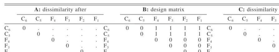
TABLE1. Matrices constructed for the partial Mantel tests for a fragmentation effect.
A: dissimilarity after
C6 C5 F4 F3 F2 F1
B: design matrix
C6 C5 F4 F3 F2 F1
C: dissimilarity before
C6 C5 F4 F3 F2 F1
C6
C5
F4
F3
F2
F1
0 .
0 . . 0
. . . 0
. . . . 0
. . . . . 0
C6
C5
F4
F3
F2
F1
0 0
0 1 1 0
1 1 0 0
1 1 0 0 0
1 1 0 0 0 0
C6
C5
F4
F3
F2
F1
0 .
0 . . 0
. . . 0
. . . . 0
. . . . . 0
Notes: Cidesignates a control, while Fidesignates a fragment, wherei indexes the replicates indicated in Fig. 2. Dots
indicate dissimilarity values calculated from the data.
examine the effects of fragmentation on species com-position and relative abundance, we used an approach based on dissimilarity measures. We asked whether communities in the fragments became more dissimilar from the controls after fragmentation, or became more similar to communities in the pine matrix after frag-mentation. Two dissimilarity measures were used. We used the Bray-Curtis measure (Bray and Curtis 1957) to measure the dissimilarity in relative abundance. The Bray-Curtis measure is widely used in community stud-ies and has been shown to provide a robust estimate of the difference in structure between communities (Faith et al. 1987). It is most sensitive to differences in the relative abundance of species between commu-nities, although it is also affected by species richness and species composition. We used the Sorensen-Czek-anowski measure (CzekSorensen-Czek-anowski 1913, Digby and Kempton 1987) to measure the dissimilarity in species composition (i.e., the presence–absence pattern). The Sorensen-Czekanowski measure is closely related to the Bray-Curtis measure but it is based only on pres-ence–absence data. It is most sensitive to species com-position but is also affected by species richness.
We used Mantel tests to determine whether com-munities in the fragments became more dissimilar from the controls after fragmentation, for each of species composition and relative abundance. To do this, we first constructed a 636 symmetric matrix of the dissimi-larity between pairs of control and fragment sites (ma-trix A, Table 1). In other words, the dissimilarity was between replicates (Table 1, Fig. 2) but calculated at the site level. Since more than one site was contrasted between two replicates, we computed all pairwise similarities and took the average to construct the dis-similarity matrix. Although the diagonal elements of A are positive when averaged at the site level, they are not informative and we set them to zero (Table 1). We constructed one matrix for each combination of size, edge, and year after fragmentation (30 combinations for each of slope and drainage line habitats). Thus, taking one combination as an example, we computed the F4-C6dissimilarity (Table 1) as the average
dissim-ilarity between (1) sites in C6classed as medium, outer,
drainage lines, for 1990, and (2) sites in F4of the same
class. We constructed a second 636 symmetric matrix
specifying the experimental design (Fortin and Gur-evitch 1993, Legendre and Legendre 1998), which we coded 0 for each within-treatment dissimilarity, and 1 for each between-treatment dissimilarity (matrix B, Ta-ble 1). The experiment has six replicates (two controls, four fragments), which gives eight possible fragment-to-control (i.e., between treatment) contrasts and seven possible (nondiagonal) within-treatment contrasts (Ta-ble 1). We constructed a third 636 dissimilarity matrix for the pre-fragmentation data, for each combination of habitat type, size, and edge, taking the site-level dissimilarity averaged over the two years (matrix C, Table 1).
To test for an effect of fragmentation on species com-position and relative abundance we computed the par-tial Mantel statisticrAB.C(the correlation between ma-trix A and B, given C). This statistic describes the effect of the fragmentation treatment on community structure when spatial variation in community structure across the site before fragmentation is removed. A pos-itive value forrAB.Cindicates an effect of fragmentation (i.e., the between-treatment dissimilarity is greater than the within-treatment dissimilarity), whereasrAB.Cequal to or less than zero indicates no effect. We conducted partial Mantel tests for positiverAB.Cby the first method of Smouse et al. (1986), using the algorithm given in Legendre and Legendre (1998:558). For each test, we used 9999 permutations and calculated the one-tail per-mutation probabilities. We conducted separate tests for each combination of size, edge, and year, as well as tests for an overall effect of fragmentation (i.e., aver-aged over site and edge).
[image:5.612.57.505.65.148.2]TABLE2. Matrices constructed for the partial Mantel tests of whether fragments were more similar to pines than controls were to pines.
D: dissimilarity
P4 P3 P2 P1
E: design matrix
P4 P3 P2 P1
F: distance
P4 P3 P2 P1
C6 C5 F4 F3 F2 . . X . . . . . X . . . . . X . . . . . C6 C5 F4 F3 F2 1 1 X 0 0 1 1 0 X 0 1 1 0 0 X 1 1 0 0 0 C6 C5 F4 F3 F2 2 1 0 1 2 3 2 1 0 1 4 3 2 1 0 5 4 3 2 1 F1 P4 P3 P2 P1 . 0 . . 0 . . . 0 X . . . 0 F1 P4 P3 P2 P1 0 — 0 — — 0 — — — X — — — — F1 P4 P3 P2 P1 3 0 2 1 0 1 2 1 0 0 3 2 1 0
Notes: Cidesignates a control, Fia fragment, and Pipines, where i indexes the replicates
indicated in Fig. 2. Dots indicate dissimilarity values calculated from the data. X indicates excluded values. Dashes indicate that coding was not applicable for the Mantel tests.
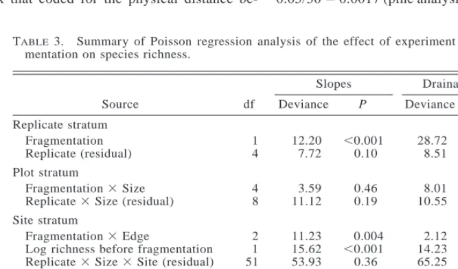
TABLE3. Summary of Poisson regression analysis of the effect of experiment forest frag-mentation on species richness.
Source df Slopes Deviance P Drainage lines Deviance P Replicate stratum Fragmentation Replicate (residual) 1 4 12.20 7.72 , 0.001 0.10 28.72 8.51 , 0.001 0.07 Plot stratum
Fragmentation3Size Replicate3Size (residual)
4 8 3.59 11.12 0.46 0.19 8.01 10.55 0.09 0.23 Site stratum
Fragmentation3Edge
Log richness before fragmentation Replicate3Size3Site (residual)
2 1 51 11.23 15.62 53.93 0.004 ,0.001 0.36 2.12 14.23 65.25 0.35 ,0.001 0.09 Year stratum Year
Year3Fragmentation Year3Fragmentation3Edge Residual 4 4 8 272 65.02 3.91 10.91 177.59 ,0.001 0.42 0.21 37.58 5.45 5.30 195.11 ,0.001 0.25 0.73
Total 359 372.85 412.32
as a site-level average. Matrix D is an extension of A to include contrasts involving pines. The question of whether communities in the fragments were more sim-ilar to the pines than the controls were to the pines involves only the upper part of matrix D (the pine– fragment and pine–control contrasts). We computed also the pine–pine contrasts, although these were not involved in any Mantel tests. As above, we constructed one matrix for each combination of size, edge, and year after fragmentation (24 combinations in each habitat type). We omitted 1987 because trapping did not begin in the pines until half way through the sampling year. We constructed a second matrix specifying the exper-imental design, which we coded 0 for each pine–frag-ment dissimilarity and 1 for each pine–control dissim-ilarity (matrix E, Table 2). We excluded within-repli-cate pine–fragment contrasts because these were not possible for pine–control contrasts. We constructed a third matrix that coded for the physical distance
be-tween replicates (matrix F, Table 2) to account for spa-tial structure (Fortin and Gurevitch 1993). To test whether fragments were more similar to the pines than controls to the pines, we computed the partial Mantel statisticrDE.F. As mentioned, this was done only for the upper part of D, E, and F. This statistic describes the degree to which the fragments were more like the pines after accounting for spatial structure. A positive value for rDE.Findicates that the fragments were more like the pines than the controls were like the pines, whereas
rDE.Fequal to or less than zero indicates no effect. We conducted partial Mantel tests as described previously. Using this approach, the experiment-wise Type I er-ror rate is inflated because multiple tests were made. We applied a Bonferroni correction to the significance level (nominallyP, 0.05) to obtain a corrected sig-nificance level. For the tests involving size and edge combinations, the corrected significance level wasP,
[image:6.612.110.448.72.192.2] [image:6.612.114.448.490.686.2]and for fragmentation overall, the significance level wasP, 0.05/5 50.01 (pine analysis P , 0.05/45 0.0125). However, the Bonferroni correction is too con-servative for a large number of tests, so we interpreted Mantel tests with uncorrected permutation probability
,0.05 as providing cautious support for the effect of fragmentation and those less than the Bonferroni cor-rected level as providing strong support.
Turnover
We calculated percentage turnover from year to year as
Cobs1Eobs
3100 (1)
Si1Si11
whereSi is the number of species at a site in year i,
Cobsis the number of species present in yeari11 but
not in year i (i.e., the number of species observed to
colonize) andEobs is the number of species absent in
year i 1 1 but present in year i (i.e., the number of
species observed to become extinct). Eq. 1 is equivalent to the Sorensen-Czekanowski dissimilarity measure, wherei indexes sites instead of years. We tested for
the effects of fragmentation, size, edges, and year on turnover using ANOVA, separately for each habitat type. We specified the error structure as a split-split-split plot as for the species richness analysis. We used a Greenhouse-Geisser adjustment to adjust probabili-ties in the year stratum for repeated measures (Green-house and Geisser 1959, von Ende 1993). Turnover between the two years before fragmentation was used as a covariate to control for spatial variation in turnover across the landscape before fragmentation.
Individual species change in occurrence by traits
We conducted an analysis of the responses of the 325 species to determine the effect of three traits: nat-ural abundance, isolation, and trophic group. For each species, the effect size was calculated as
pfragments2 pcontrols (2)
wherepfragments is the probability of occurrence in the
fragments andpcontrolsis the probability of occurrence
in the controls. The effect size was calculated for each of six treatment types (fragment edge, small-fragment interior, medium edge, medium interior, large edge, large interior). To calculatepfragmentswe first
cal-culated the mean probability of occurrence in each of these treatment types for each post-fragmentation year (five years) and then calculated the mean of the annual values. We calculatedpcontrolsin the same way but did
not calculate the probability of occurrence separately for each treatment type in order to give a larger sample size. The effect size was either positive or negative depending on whether a species had become more, or less, likely to occur in a given treatment type (e.g., small interior sites) than in the controls.
Regressing effect size against traits of species.—
Three traits of species were considered. A fourth, body size, was tested in a previous analysis of traits by change in abundance and was not significant (Davies et al. 2000) so it was not considered here.
1. Natural abundance.—For each species, we summed catches for the two years of sampling that took place before the fragmentation treatment was applied. 2. Isolation.—In the absence of dispersal
informa-tion, we calculated instead an isolation index for each species by dividing the number of individuals caught in the pine matrix (44 sites) by the number caught in the fragments (96 sites), post-fragmentation, after first equalizing the data for trapping effort. Beetles fell into two categories. (1) Never trapped in the pine matrix (isolated). For a species to be isolated two conditions were necessary: (a) the species did not occur in the matrix. That is, the species was a habitat specialist of eucalypt habitat, and (b) the species did not disperse between fragments. Given that roughly one-quarter of the trapping effort was in the matrix, we are confident that if a species was not caught in the matrix in five years of trapping, it did not occur there. Similarly, we are confident that these species did not disperse along the ground through the matrix, or rarely did so. Un-fortunately, we can say little about other modes of dis-persal. Thus, it is possible that some species catego-rized as isolated met the first condition but were able to disperse, undetected, between fragments. (2) Trapped in the pine matrix (not isolated). These species either had populations established in the pine matrix (were habitat generalists), or dispersed through the ma-trix between fragments. Given these caveats, we be-lieve that these isolation categories are useful as a first approximation, particularly given that the contrasts that we make are relative rather than absolute.
3. Trophic group.—Beetles were assigned to one of
four trophic groups: (a) species feeding on detritus and deadwood (hereafter referred to as detritivores), (b) fungivores, (c) herbivores, and (d) predators. Depend-ing on the knowledge of the species, the assignments were made at the species or genus or, in some cases, subfamily level by J. F. Lawrence (Australian National Insect Collection, CSIRO Entomology, Canberra).
We used multiple regression to test for the effects of these three traits on the responses of beetles to frag-mentation in different parts of the experiment (small edges, small interiors, medium edges, medium interi-ors, large edges, large interiors). The effect size was weighted by total occurrence before fragmentation so that less weight was placed on the responses of those species that occurred only a few times. Model fitting took place as follows. First, the full model was fitted including the three traits as variables. Each variable was dropped from the full model one at a time and then replaced.P values were calculated from variance
ratios and a variable was considered significant when
model assumptions were determined by viewing his-tograms of the data, plots of residuals vs. fitted values, and plotting residuals as a normal order probability plot.
RESULTS
The structure of the beetle community was signifi-cantly different in slope compared to drainage line hab-itat for all measures (richness, Poisson regression, P 50.001; species composition, Mantel test,P,0.001; relative abundance, Mantel test,P, 0.001, turnover, ANOVA,P , 0.001). In all subsequent analyses, we considered slopes and drainage lines separately.
Species richness
There was a significant effect of habitat fragmen-tation on species richness (Table 3). In slope habitat, species richness increased by one to two species per site at fragment edges compared to fragment interiors and continuous forest (Fig. 3, Table 3), but there was no effect of fragment size (Table 3, Fragment3Size). The pattern in species richness on slopes corresponds with the model for an edge effect that penetrates 20 m or less (contrast Fig. 1a and Fig. 3). That is, only edges were affected in all fragment sizes, not interiors. In the drainage line habitat, species richness increased slight-ly in fragments compared to controls but there was no effect of fragment size or of edges (Table 3). For both slopes and drainage lines, removing new colonizers (species not present in the landscape before fragmen-tation) from the analyses had no effect on these results. Thus, the increase in richness at fragment slope edges and in fragment drainage lines was not explained by new species colonizing from the matrix.
Species composition
Species composition changed significantly in frag-ments compared to continuous forest (Fig. 3, Table 4). However, in drainage line habitat a significant effect was observed only for small edges in 1988 (Table 4). In slope habitat, the change in composition was greatest in years 1989 and 1990 (3–4 yr post-fragmentation). For these years, there was a tendency for small frag-ments to be most different from controls and for large interior sites to be most similar to controls (Fig. 3). Thus, in years 1989 and 1990, the pattern was consis-tent with a 50–100 m edge effect (contrast Fig. 1c and Fig. 3 slope habitat).
Relative abundance
Changes in the relative abundance of species due to habitat fragmentation were more pronounced than changes in species composition (Fig. 3). The biggest effects of fragmentation were observed in slope habitat. In slope habitat, a significant effect of fragmentation was observed for years 1988–1991 (Table 4) and was greatest in 1989 and 1990 (Fig. 3). Significant changes in relative abundance were also detected in drainage
line habitat, where small and medium fragments were significantly different from controls in years 1989 to 1991 (Fig. 3, Table 4). Differences due to fragment size and edge effects in both habitats did not become ap-parent until three years post-fragmentation (1989), when small and medium fragments were most different from controls and large fragments were most similar to controls (Fig. 3). For slopes, the pattern in relative abundance corresponded to model predictions for an edge effect that penetrated 100 m (contrast Fig. 1c and Fig. 3 slope habitat).
Turnover
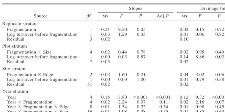
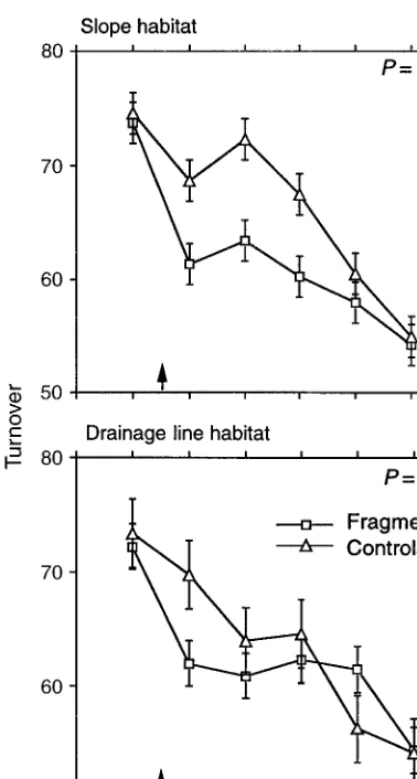
Fragmentation significantly reduced species turnover in slope habitat but not in drainage line habitat (Table 5, Fig. 4). This was set against a decline in turnover over the period of the experiment, in both fragments and controls (Fig. 4). Turnover was significantly dif-ferent from year to year (Table 5). There were no size or edge effects on species turnover (Table 5).
The matrix
There were three results. First, in many later years, the species composition and relative abundance of sites in the pine matrix were more like the fragments than the controls were like the pine matrix (Fig. 5) although the difference was significant only in some years and more often in drainage lines (Table 6). Second, in drain-age line habitat in the later years, the species compo-sition and relative abundance of small-fragment edges were most like the matrix and large-fragment interiors were least like the matrix (Fig. 5). This pattern cor-responded to model predictions for an edge effect that penetrated 50–100 m (contrast Fig. 1c and Fig. 5 drain-age line habitat). In slope habitat, while the species composition and relative abundance of fragments were most like the matrix in some years, averaged over all size and edge classes (Table 6), there did not appear to be a consistent pattern related to size or edge (Table 6, Fig. 5). Third, species richness was significantly low-er at matrix sites than at fragment and continuous forest sites, by one to two species (Poisson regression,P5
0.002, Fig. 3).
Individual species responses and traits
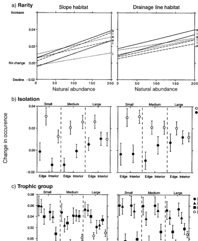
Rarity.—Natural abundance affected the responses
of species to fragmentation (Fig. 6, Table 7). Species with high natural abundances increased in occurrence in fragments compared to continuous forest, while rare species were not affected. The relationship between rarity and response to fragmentation was not different in different parts of the fragmented landscape (e.g., small-fragment edges vs. large-fragment interiors).
Isolation.—Species that were not isolated increased
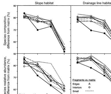
FIG. 3. Effects of experimental fragmentation, fragment size, and edges on species richness, species composition, and species relative abundance, over seven years. For species composition (presence–absence) and relative abundance, the dark lines are the average fragment-control dissimilarity (from A, Table 1), for each combination of habitat type (slopes, drainage lines), fragment size, and edge. The gray lines are the average within-treatment dissimilarity (from A, Table 1), further averaged across sizes and edges. The gray lines thus represent the expected pattern for the null hypothesis of no fragmentation effect. Dissimilarities after fragmentation shown here are not adjusted for dissimilarity before fragmentation. Arrows indicate when fragmentation occurred. Significance levels appear in Table 4.
small declines in the occurrence of species in small fragments and at medium-fragment edges (Fig. 6).
Trophic group.—There was a significant effect of
trophic group on species’ responses to fragmentation (Table 7). Detritivores and fungivores occurred at more sites post-fragmentation but occurrences of herbivores
were variable, while predators occurred at fewer sites post-fragmentation (Fig. 6).
Evidence of a deeply penetrating edge effect.—For
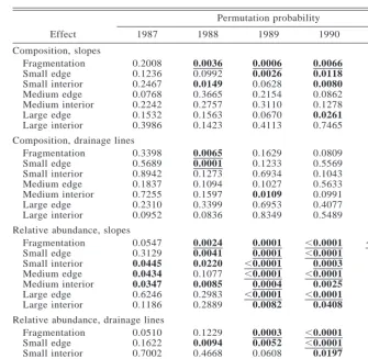
TABLE4. Randomization significance levels for the effects of forest fragmentation on species composition and relative abundance, for slope and drainage line habitat.
Effect
Permutation probability
1987 1988 1989 1990 1991
Composition, slopes Fragmentation Small edge Small interior Medium edge Medium interior Large edge Large interior 0.2008 0.1236 0.2467 0.0768 0.2242 0.1532 0.3986 0.0036 0.0992 0.0149 0.3665 0.2757 0.1563 0.1423 0.0006 0.0026 0.0628 0.2154 0.3110 0.0670 0.4113 0.0066 0.0118 0.0080 0.0862 0.1278 0.0261 0.7465 0.0094 0.0953 0.3565 0.1374 0.7854 0.0445 0.0439
Composition, drainage lines Fragmentation Small edge Small interior Medium edge Medium interior Large edge Large interior 0.3398 0.5689 0.8942 0.1837 0.7255 0.2310 0.0952 0.0065 0.0001 0.1273 0.1094 0.1597 0.3399 0.0836 0.1629 0.1233 0.6934 0.1027 0.0109 0.6953 0.8349 0.0809 0.5569 0.1043 0.5633 0.0991 0.4077 0.5489 0.0706 0.1082 0.3663 0.3318 0.4587 0.1734 0.3397 Relative abundance, slopes
Fragmentation Small edge Small interior Medium edge Medium interior Large edge Large interior 0.0547 0.3129 0.0445 0.0434 0.0347 0.6246 0.1186 0.0024 0.0041 0.0220 0.1077 0.0085 0.2983 0.2889 0.0001 0.0001 ,0.0001 ,0.0001 0.0004 ,0.0001 0.0082 ,0.0001 ,0.0001 0.0003 ,0.0001 0.0025 ,0.0001 0.0408 ,0.0001 0.0001 0.1259 0.0045 0.0003 0.1052 0.1954 Relative abundance, drainage lines
Fragmentation Small edge Small interior Medium edge Medium interior Large edge Large interior 0.0510 0.1622 0.7002 0.0279 0.5879 0.0581 0.0325 0.1229 0.0094 0.4668 0.4297 0.0910 0.5395 0.7799 0.0003 0.0052 0.0608 0.0028 ,0.0001 0.3146 0.8130 ,0.0001 ,0.0001 0.0197 0.0421 0.0002 0.1920 0.7485 0.0027 0.0004 0.0015 0.4237 0.0315 0.0519 0.1714
Notes: Permutation probabilities are the proportions of times that the partial Mantel statistic
obtained by random permutation exceeded the observed partial Mantel statistic. Bold values indicate permutation probability,0.05. Underlined values indicate permutation probability less than the Bonferroni-corrected Type I error rate.
m). This gradient corresponded with the changes seen in the community-level measures, in relative abun-dance and to a smaller extent in species composition, which were greatest at fragment edges and small-est in large-fragment interiors (Figs. 3 and 5).
DISCUSSION
There were four main findings. First, experimental forest fragmentation affected species composition, rel-ative abundance, and richness via two edge effects with different penetration distances. The pattern of change in species composition and species relative abundance corresponded with a deeply penetrating edge effect (to 100 m). That is, changes were generally greatest at small-fragment edges and negligible at large-fragment interiors. Species richness increased slightly at slope edges but there was no fragment-size effect, corre-sponding with model predictions for a shallowly pen-etrating edge effect (to 20 m). Second, fragmentation reduced species turnover. Further, changes in turnover and the other measures of community structure
(rich-ness, composition, relative abundance) were set against large background spatial and temporal variation in community structure that declined over the period of the experiment reported here. Third, matrix sites were more like fragments than continuous forest sites, in species composition and relative abundance, and they were less species rich than fragment and continuous-forest sites. In drainage line habitat, small-edge sites were most like the matrix and large interior sites were least like the matrix. This pattern of change also cor-responds with a deeply penetrating edge effect. Fourth, changes in the occurrences of individual species were linked to rarity, degree of isolation, and trophic group, and these changes in occurrence also tended to be great-est at small-fragment edges and smallgreat-est at large-frag-ment interiors.
[image:10.612.112.447.73.400.2]TABLE5. Repeated-measures ANOVA of the effect of experimental forest fragmentation on species turnover.
Source df
Slopes
MS F P AdjP
Drainage lines
MS F P AdjP
Replicate stratum Fragmentation
Log turnover before fragmentation Residual
1 1 3
0.21 0.03 0.02
9.50 1.29
0.05 0.33
0.02 0.01 0.10
0.15 0.06
0.72 0.82
Plot stratum
Fragmentation3Size
Log turnover before fragmentation Residual
4 1 7
0.02 0.00 0.05
0.44 0.03
0.78 0.87
0.02 0.14 0.02
0.95 8.86
0.49 0.02
Site stratum
Fragmentation3Edge
Log turnover before fragmentation Residual
2 1 51
0.03 0.00 0.02
1.60 0.00
0.21 1.00
0.04 0.01 0.02
3.02 0.79
0.06 0.38
Year stratum Year
Year3Fragmentation Year3Fragmentation3Edge Year3Fragmentation3Size Residual
4 4 8 16 256
0.15 0.02 0.01 0.01 0.01
17.80 2.24 1.34 1.08
,0.001 0.07 0.22 0.38
,0.001 0.11 0.34 0.55
0.12 0.02 0.01 0.01 0.01
9.32 2.16 0.98 0.85
,0.001 0.07 0.45 0.63
,0.001 0.12 0.59 0.78
Total 359
Note: Greenhouse-Geisser adjusted probabilities (‘‘Adj P’’) are given for the year stratum.
discuss within-patch processes and between-patch pro-cesses in more detail.
Within-patch processes
Hypothesis 1 predicted that species richness would be reduced as a result of an increased extinction risk in small populations on fragments. Contrary to this prediction, species richness increased (Fig. 3, discussed further in relation to hypothesis 2). Further, at the spe-cies level there was little evidence of an increase in extinction rate since the occurrence of rare species was not affected by fragmentation (Fig. 6). Previously we found that rare species declined in abundance in frag-ments compared to continuous forest (Davies et al. 2000), suggesting that fragmentation affected the abun-dance but not the occurrence of rare species. Never-theless, those declines in abundance may in time be-come changes in species occurrences.
In support of hypothesis 2, edge effects altered the occurrences and abundances of species on fragments compared to continuous forest. Two edge effects, with different penetration distances, changed the structure of the beetle community. One penetrated a short dis-tance and altered species richness in slope habitat while the other penetrated deeply and affected species rela-tive abundance in both slope and drainage line habitats and, to a lesser extent, species composition in slope habitat.
A shallow edge effect in richness.—In slope habitat,
species richness increased by 1–2 species, at fragment edges, in all fragment sizes, consistent with model pre-dictions for an edge effect that penetrated 20 m (com-pare Fig. 3 and Fig. 1a). This was probably not the result of the colonization of fragment edges by species
from the matrix because the species composition of slope fragment edges was no more like the matrix than fragment interiors (Fig. 5). Neither was the increase due to species that were new to the landscape. Thus, the extra species at slope edges came from within the fragments themselves. The change in richness at edges may have resulted from habitat modification at edges. Slope habitat is characterized by open eucalypt forest so, for example, productivity may have increased at edges as the result of an increase in solar radiation.
In contrast, in drainage line habitat, species richness increased by 1–2 species in fragments compared to continuous forest but there was no difference in effect between edge and interior sites. The vegetation in drainage lines is different from the slope habitat, so it is not surprising that there is a different result between the two habitats. However, in addition to the vegetation being different, drainage lines also have a hydrological function in the landscape. There is anecdotal evidence that the hydrology of fragment drainage lines was al-tered when the land surrounding the fragments was cleared and that they now experience greater fluxes of water than the continuous forest controls. Since these changes result from landscape-wide alterations, they might be expected not to exhibit edge effects. However, it is not clear that such hydrological changes are linked to the increase in species richness.
[image:11.612.60.500.64.283.2]spe-FIG. 4. Mean turnover (percentage change in species com-position) from one year to the next for sites in fragments and continuous forest. Means and standard errors are from ANOVA. The arrows indicate when fragmentation occurred.
P values are for the significance of the difference between
fragments and controls after fragmentation. There was not a significant effect of fragment size or edges.
cies richness of flowering plants and insects increased with increasing habitat subdivision (Quinn and Rob-inson 1987).
However, many studies have reported declines in richness as the result of fragmentation. In the Brazilian experiment, the richness of insectivorous birds (Stouf-fer and Bierregaard 1995) and of dung and carrion bee-tles (Klein 1989) declined with isolation. In scrub hab-itat fragments in southern California, ant species rich-ness was lower in smaller fragments (Saurez et al. 1998). In subtropical dry forest in northwest Argentina, the richness of native flower visitors was lower in smaller fragments (Aizen and Feinsiger 1994). In a Kansas oldfield, larger patches were more species rich than small patches (Holt et al. 1995).
A deeply penetrating edge effect in relative abun-dance and composition.—A pattern consistent with
model predictions for a deeply penetrating edge effect occurred in (1) changes in species’ relative abundance and composition (Fig. 3), and (2) as increases and de-clines in individual species’ occurrences by trophic group and degree of isolation (Fig. 6). The degree of change for each combination of fragment size and edge was close to the pattern predicted by the model for an edge effect that penetrated;100 m (Fig. 1c). That is, changes were largest at small-fragment edges and neg-ligible at large-fragment interiors. This pattern was strongest for changes in the relative abundance of spe-cies in the beetle community. The pattern was also present for species composition. The edge effect had a greater impact on species’ abundance than on their occurrence.
We hypothesize that habitat modification is the main cause of this edge effect, although the exact form of modification is not clear. For example, the edge effect was evident as increases in the occurrence of detriti-vores and fungidetriti-vores (Fig. 6). This may have been in response to an increase on the forest floor of litter and dead wood, and thus also fungal spores. Although there was visual evidence of increased windthrow at frag-ment edges, we have not yet docufrag-mented this empir-ically. Nonetheless, in another forest fragmentation ex-periment at Manaus in Brazil, edge effects that altered microclimate and increased wind turbulence near edges were considered the most important cause of increased tree mortality and damage in rain forest fragments (Laurance et al. 1998).
The effects of altered forest structure and microcli-mate have also been documented in the Brazilian ex-periment as greater changes in community structure of small than large fragments. Like our findings, beetle community structure (relative abundance) was affected by fragment size and edges and was most different from continuous forest in the smallest fragments (Didham et al. 1998). For insectivorous bird communities, the rel-ative abundance of 1-ha fragments diverged more from pre-fragmentation communities than did 10-ha frag-ments (Stouffer and Bierregaard 1995). In the dung and carrion beetle community, the relative abundance of spe-cies in small and large fragments was different and both sizes were different from continuous forest (Klein 1989).
Between-patch scales
[image:12.612.62.271.46.436.2]FIG. 5. Mean difference in species composition (presence–absence) and relative abundance of sites in the pine matrix compared to other sites. Three dissimilarities were computed: pine matrix vs. control, pine matrix vs. fragment, and pine matrix vs. pine matrix. For species composition and relative abundance, the dark lines are the average fragment–matrix dissimilarity (from D, Table 2), for each combination of habitat type (slopes, drainage lines), fragment size, and edge. The gray lines are the average control–matrix dissimilarity (from D, Table 2), further averaged across sizes and edges. The gray lines thus represent the expected pattern for the null hypothesis of no fragmentation effect. Departures in the downward direction from the gray line indicate that fragment sites were more similar to matrix sites than control sites were to matrix sites. The matrix–matrix comparison represents the spatial variability in community structure among sites in the matrix (average from D, Table 2). Significance levels appear in Table 6.
There are two possible reasons for these findings. First, dispersal between fragments was reduced, af-fecting abundance (e.g., Hanski et al. 1994), but not enough time had elapsed for extinctions to occur. This explanation highlights a problem common to fragmen-tation experiments conducted at landscape scales, that processes contributing to extinction within fragments operate over time scales longer than most fragmenta-tion experiments have been running. Extincfragmenta-tion events that result from environmental stochasticity, demo-graphic stochasticity, or loss of genetic variation are more likely to be observed over decades than years.
Second, dispersal between fragments was not re-duced because the matrix was not inhospitable to ment-inhabiting species (hypothesis 4). Many frag-ment-inhabiting species occurred in the matrix, in some cases in high abundances (Davies et al. 2000). Further, species that were captured in the matrix were captured at more sites in fragments than in continuous forest;
that is, they increased their occurrence within frag-ments. Species that were abundant in the matrix also increased in abundance on fragments compared to con-tinuous forest (Davies et al. 2000). Thus, for many species, the effect of modifying the landscape may have been to reduce the probability of extinction within frag-ments by increasing the net flow of individuals in to fragments. Our findings support predictions from a me-tacommunity model that species that are abundant in the common habitat (matrix) have potential to become more common members of local communities in the sparser habitat (fragments) than species that do not inhabit the common habitat (Holt 1997).
[image:13.612.84.471.48.374.2]TABLE6. Randomization significance levels for whether the species composition and relative abundance of fragments were more similar to the pine matrix than controls were to the pine matrix, for slope and drainage line habitat.
Effect
Permutation probability
1988 1989 1990 1991
Composition, slopes Fragmentation Small edge Small interior Medium edge Medium interior Large edge Large interior 0.4086 0.5975 0.5620 0.3986 0.1925 0.3003 0.5218 0.1238 0.0443 0.0631 0.2213 0.3755 0.1327 0.2984 0.2507 0.2066 0.2642 0.0964 0.1977 0.9549 0.2113 0.0244 0.1181 0.0293 0.4993 0.3510 0.0362 0.2284 Composition, drainage lines
Fragmentation Small edge Small interior Medium edge Medium interior Large edge Large interior ,0.0001 0.0042 0.0523 0.0004 0.0637 0.0010 0.0048 0.2731 0.0193 0.7135 0.5610 0.0035 0.4415 0.9752 0.0021 0.3478 0.0020 0.0133 0.0007 0.1404 0.2172 0.0930 0.8043 0.2359 0.1779 0.6219 0.0201 0.0603 Relative abundance, slopes
Fragmentation Small edge Small interior Medium edge Medium interior Large edge Large interior 0.7471 0.6563 0.7385 0.8837 0.7732 0.6307 0.6235 0.0797 0.0254 0.0013 0.0435 0.6417 0.6673 0.0708 0.0002 0.0183 0.0005 0.0001 0.0020 0.0064 0.0090 0.1356 0.3925 0.0833 0.6055 0.4240 0.1433 0.0133
Relative abundance, drainage lines Fragmentation Small edge Small interior Medium edge Medium interior Large edge Large interior 0.8345 0.9489 0.6962 0.6519 0.9237 0.7381 0.5806 0.0335 0.0931 0.1090 0.0724 0.0112 0.0185 0.5674 0.0275 0.1727 0.0427 0.0424 0.0028 0.0549 0.2452 ,0.0001 0.0013 0.0035 0.0703 0.0036 0.0002 0.0184
Notes: Permutation probabilities are the proportions of
times that the partial Mantel statistic obtained by random permutation exceeded the observed partial Mantel statistic. Bold values indicate permutation probability,0.05. Under-lined values indicate permutation probability less than the Bonferroni-corrected Type I error rate.
in extinction rate or to a change in colonization rate because these rates are not the same asEobsandCobsin
Eq. 1. For example, the number of species observed to go extinct in one period (Eobs) depends on both the true
extinction rate and the colonization rate. However, since turnover results from the net effect of extinction and colonization, the fact that turnover changed means that one or both of these rates was altered by frag-mentation. Paradoxically, our other results suggest that either the extinction rate was reduced or the coloni-zation rate increased, since the occurrences of species within fragments increased.
Turnover appeared to be independent of habitat mod-ification because there were no edge or size effects in turnover, which is in contrast to Bengtsson et al. (1997) who found that habitat stability contributed to com-munity stability in British woodland birds. Three stud-ies have recorded increased community variability as
the result of habitat fragmentation. Holt et al. (1995) found that spatial heterogeneity in vegetation compo-sition increased in grassland patches, less so in large patches. Boulinier et al. (1998) found that temporal variability in the richness of forest breeding birds in-creased as the result of higher local extinction rates. Finally, Laurance et al. (1998) found that tree turnover was significantly higher at the edges of 18-yr-old trop-ical rain forest fragments, as the result of increased mortality.
IMPORTANTCONSIDERATIONS
Two final points deserve consideration. First, the ef-fects of fragmentation on community structure were set against high natural spatial and temporal variability in community structure. Spatial and temporal variability in community structure declined over the period of the experiment (1985–1991). That is, the species compo-sition and relative abundance of species in the frag-ments, continuous forest, and the matrix became more similar from site to site (reduced spatial variation, Fig. 3) and more similar from year to year (reduced tem-poral variability, Fig. 4). This inherent temtem-poral and spatial variability in community structure highlights the necessity of long-term, controlled and replicated field experiments. For example, had our experimental design included only before and after data, with no controls, we would have reached very different con-clusions.
[image:14.612.57.271.90.417.2]FIG. 6. Change in occurrence of individual species in fragments compared to continuous forest, regressed against traits of species (n5325): (a) rarity, (b) degree of isolation, and (c) trophic group. A change in occurrence of 0.02, for example, means that species occurred at 2% more sites in the fragments than in the controls. Change in occurrence was calculated for three fragment sizes (small, medium, and large), at fragment edges and interiors. For (a), small dashes are small fragments, large dashes are medium fragments, and hard lines are large fragments; e5edge, and i 5interior. Error bars represent standard errors. Significance levels appear in Table 7.
on a timescale of months, individuals rarely move fur-ther than 10 m.
CONCLUSIONS
We set out to determine which population-level pro-cesses were altered and thus changed the structure of
TABLE7. Summary of multiple regression analyses of individual species changes in occurrence and their traits for three fragment sizes at fragment edges and interiors.
Source df Small edge F P Small interior F P Medium edge F P Medium interior F P Large edge F P Large interior F P Slope habitat Rarity Isolation Trophic Error 1 1 3 288 1.60 12.23 28.02 0.21 ,0.001 ,0.001 0.15 6.97 20.86 0.70 0.009 ,0.001 2.34 9.77 12.57 0.13 0.002 ,0.001 12.55 27.56 22.73 ,0.001 ,0.001 ,0.001 20.88 17.96 23.16 ,0.001 ,0.001 ,0.001 75.51 2.31 19.88 ,0.001 0.12 ,0.001 Drain habitat Rarity Isolation Trophic Error 1 1 3 288 2.13 3.22 20.58 0.15 0.07 ,0.001 1.41 6.84 28.48 0.23 0.009 ,0.001 0.04 8.07 33.77 0.84 0.005 ,0.001 1.48 1.54 31.02 0.23 0.22 ,0.001 4.35 7.17 25.90 0.04 0.008 ,0.001 11.88 2.35 20.21 ,0.001 0.13 ,0.001
but it was too early to detect their consequences. In-stead, edge effects had an overwhelming influence on community structure at the within-fragment scale. Pro-cesses operating at the between-fragment scale were less important, supporting the suggestion that the role of local processes in regional persistence may have been underemphasized (Harrison and Taylor 1997, Har-rison and Bruna 1999). Unexpectedly, turnover de-clined on fragments compared to continuous forest, ei-ther as the result of a reduction in extinction rate or an increase in the colonization rate, or both. Further, the matrix had a stabilizing role on the fragment com-munity by allowing species that could persist in the matrix to increase their occurrences within fragments.
ACKNOWLEDGMENTS
John Lawrence spent an enormous amount of time iden-tifying the beetle fauna, for which we are very grateful. We thank Julian Ash, Edward F. Connor, Penny Gullan, and two reviewers for their comments, which greatly improved the manuscript. We thank Ross Cunningham and Christine Don-nelly, who provided statistical and programming advice, and George Milkovits who manages the experiment. We also thank all of the people who have helped out in the field over the years. Finally, we thank State Forests of New South Wales for their cooperation and assistance. Kendi Davies and Brett Melbourne were supported by Australian Postgraduate Awards.
LITERATURECITED
Aizen, M. A., and P. Feinsinger. 1994. Forest fragmentation, pollination and plant reproduction in a Chaco dry forest, Argentina. Ecology 75:330–351.
Austin, M. P., and A. O. Nicholls. 1988. Species associations within herbaceous vegetation in an Australian eucalypt for-est. Pages 95–114in H. J. During, M. J. A. Werger, and J.
H. Willems, editors. Diversity and pattern in plant com-munities. SPB Academic Publishing, The Hague, The Neth-erlands.
Bengtsson, J., S. R. Baillie, and J. H. Lawton. 1997. Com-munity variability increases with time. Oikos 78:249–256. Boulinier, T., J. D. Nichols, J. E. Hines, J. R. Sauer, C. H. Flather, and K. H. Pollock. 1998. Higher temporal vari-ability of forest breeding bird communities in fragmented landscapes. Proceedings of the National Academy of Sci-ences (USA) 95:7497–7501.
Bray, J. R., and J. T. Curtis. 1957. An ordination of the upland forest communities of Southern Wisconsin. Ecological Monographs 27:325–349.
Czekanowski, J. 1913. Zarys metod statystycznych w zas-tosowaniu do anthropolgii. Naklad Towaraystwa Naukow-ego WarszawskiNaukow-ego, Warszawa, Poland.
Davies, K. F., and C. R. Margules. 1998. Effects of habitat fragmentation on carabid beetles: experimental evidence. Journal of Animal Ecology 67:460–471.
Davies, K. F., C. R. Margules, and J. F. Lawrence. 2000. Which traits of species predict population declines in ex-perimental forest fragments? Ecology 81:1450–1461. Diamond, J. M., K. D. Bishop, and S. van Balen. 1987. Bird
survival in an isolated Javan woodland: island or mirror? Conservation Biology 1:132–142.
Didham, R. K., P. M. Hammond, J. H. Lawton, P. Eggleton, and N. E. Stork. 1998. Beetle species responses to tropical forest fragmentation. Ecological Monographs 68:295–323. Digby, P. G. N., and R. A. Kempton. 1987. Multivariate analysis of ecological communities. Chapman and Hall, London, UK.
Fahrig, L., and G. Merriam. 1994. Conservation of frag-mented populations. Conservation Biology 8:50–59. Faith, D. P., P. R. Minchin, and L. Belbin. 1987.
Composi-tional dissimilarity as a robust measure of ecological dis-tance. Vegetatio 69:57–68.
Fortin, M.-J., and J. Gurevitch. 1993. Mantel tests: spatial structure in field experiments. Pages 342–359 in S. M.
Scheiner and J. Gurevitch, editors. Design and analysis of ecological experiments. Chapman and Hall, New York, New York, USA.
Gascon, C., T. E. Lovejoy, R. O. Bierregaard Jr., J. R. Mal-colm, P. C. Stouffer, H. Vasconcelos, W. F. Laurance, B. Zimmerman, M. Tocher, and S. Borges. 1999. Matrix hab-itat and species persistence in tropical forest remnants. Bi-ological Conservation 91:223–229.
Genstat 5 Committee. 1997. Genstat 5, release 4.1, reference manual supplement. Numerical Algorithms Group, Oxford, UK.
Greenhouse, S. W., and S. Geisser. 1959. On methods in the analysis of profile data. Psychometrika 24:95–112. Hanski, I. 1994. Patch-occupancy dynamics in fragmented
landscapes. Trends in Ecology and Evolution 9:131–135. Hanski, I., M. Kuussaari, and M. Nieminen. 1994.
Meta-population structure and migration in the butterflyMelitaea cinxia. Ecology 75:747–762.
Harrison, S., and E. Bruna. 1999. Habitat structure and large-scale conservation: what do we know for sure? Ecography
22:225–232.
Harrison, S., and A. D. Taylor. 1997. Empirical evidence for metapopulation dynamics. Pages 27–42in I. A. Hanski and
M. E. Gilpin, editors. Metapopulation biology: ecology, genetics and evolution. Academic Press, San Diego, Cal-ifornia, USA.
com-munity structure: some consequences of spatial heteroge-neity. Pages 149–164in I. A. Hanski and M. E. Gilpin,
editors. Metapopulation biology: ecology, genetics and evolution. Academic Press, San Diego, California, USA. Holt, R. D., G. R. Robinson, and M. S. Gaines. 1995.
Veg-etation dynamics in an experimentally fragmented land-scape. Ecology 76:1610–1624.
Kapos, V. 1989. Effects of isolation on the water status of forest patches in the Brazilian Amazon. Journal of Tropical Ecology 5:173–185.
Kapos, V., E. Wandelli, J. L. Camargo, and G. Ganade. 1997. Edge-related changes in environment and plant responses due to forest fragmentation in central Amazonia. Pages 33– 44in W. F. Laurance and R. O. Bierregaard, editors.
Trop-ical forest remnants: ecology, management, and conser-vation of fragmented communities. University of Chicago Press, Chicago, Illinois, USA.
Klein, B. C. 1989. Effects of forest fragmentation on dung and carrion beetle communities in central Amazonia. Ecol-ogy 70:1715–1725.
Laurance, W. F., L. V. Ferreira, J. M. Rankin-de Merona, and S. G. Laurance. 1998. Rain forest fragmentation and the dynamics of Amazonian tree communities. Ecology 79: 2032–2040.
Legendre, P., and L. Legendre. 1998. Numerical ecology. Second English edition. Elsevier, Amsterdam, The Neth-erlands.
Levins, R. 1969. Some demographic and genetic consequenc-es of environmental heterogeneity for biological control. Bulletin of the Entomological Society of America 15:237– 240.
MacArthur, R. H., and E. O. Wilson. 1967. The theory of island biogeography. Princeton University Press, Princeton, New Jersey, USA.
Malcolm, J. R. 1994. Edge effects in Central Amazonian forest fragments. Ecology 75:2438–2445.
Margules, C. R. 1993. The Wog Wog habitat fragmentation experiment. Environmental Conservation 19:316–325. Margules, C. R., G. A. Milkovits, and G. T. Smith. 1994.
Contrasting effects of habitat fragmentation on the scorpion
Cercophonius squama and an amphipod. Ecology 75:2033–
2042.
Quinn, J. F., and G. R. Robinson. 1987. The effect of ex-perimental subdivision on the flowering plant diversity in a California annual grassland. Journal of Ecology 75:837– 856.
Robinson, G. R., and J. F. Quinn. 1988. Extinction, turnover and species diversity in an experimentally fragmented Cal-ifornian annual grassland. Oecologia 76:71–82.
Saunders, D. A., R. J. Hobbs, and C. R. Margules. 1991. Biological consequences of ecosystem fragmentation: a re-view. Conservation Biology 5:18–32.
Saurez, A. V., D. T. Bolger, and T. J. Case. 1998. Effects of fragmentation and invasion on native ant communities in coastal southern California. Ecology 79:2041–2056. Sisk, T. D., and C. R. Margules. 1993. Habitat edges and
restoration: methods for quantifying edge effects and pre-dicting the results of restoration efforts. Pages 57–69in D.
A. Saunders, R. J. Hobbs, and P. R. Ehrlich, editors. Nature conservation 3: reconstruction of fragmented ecosystems, global and regional perspectives. Surrey Beatty & Sons, Chipping Norton, NSW, Australia.
Smouse, P. E., J. C. Long, and R. R. Sokal. 1986. Multiple regression and correlation extensions of the Mantel test of matrix correspondence. Systematic Zoology 35:627–632. Stouffer, P. C., and R. O. Bierregaard, Jr. 1995. Use of
Am-azonian forest fragments by understory insectivorous birds. Ecology 76:2429–2445.
von Ende, C. N. 1993. Repeated-measures analysis: growth and other time-dependent measures. Pages 113–137in S.