A full bi-tensor neural tractography algorithm using the unscented Kalman filter

R E S E A R C H

Open Access

A full bi-tensor neural tractography algorithm

using the unscented Kalman filter

Stefan Lienhard

, James G Malcolm

, Carl-Frederik Westin

and Yogesh Rathi

Abstract

We describe a technique that uses tractography to visualize neural pathways in human brains by extending an existing framework that uses overlapping Gaussian tensors to model the signal. At each point on the fiber, an unscented Kalman filter is used to find the most consistent direction as a mixture of previous estimates and of the local model. In our previous framework, the diffusion ellipsoid had a cylindrical shape, i.e., the diffusion tensor’s second and third eigenvalues were identical. In this paper, we extend the tensor representation so that the diffusion tensor is represented by an arbitrary ellipsoid. Experiments on synthetic data show a reduction in the angular error at fiber crossings and branchings. Tests on in vivo data demonstrate the ability to trace fibers in areas containing crossings or branchings, and the tests also confirm the superiority of using a full tensor representation over the simplified model.

1 Introduction

Diffusion-weighted magnetic resonance imaging has provided the opportunity for non-invasive investigation of neural architecture of the brain. Neuroscientists use this imaging technique to find out how neurons origi-nating from one region in the brain connect to other regions and how well-defined those connections are. The quality of the results of such studies relies heavily on the chosen fiber representation and the reconstruc-tion method, to trace neural pathways.

For studying the microstructure of fibers, we need a model to interpret the diffusion-weighted signal. There are two main categories for such models: parametric and non-parametric models. The simplest parametric model is the diffusion tensor describing a Gaussian esti-mate of the diffusion orientation and its strength in each voxel. Despite its robustness, this model is inade-quate in cases where several fiber populations cross, join or split in one voxel [1,2]. Several parametric models have been introduced for handling more complex diffu-sion patters such as mixtures of tensors [3-7], higher-order tensors [8], diffusion orientation transforms [9] and directional functions [10-12]. When fitting the data, one must make certain assumptions about the model. For example, the number of components present in a

particular voxel must be determined [13]. As seen in this paper, incorporating information from neighboring voxels helps in this process [14].

Usually non-parametric models contain more informa-tion about the diffusion pattern. Instead of estimating a discrete number of fibers as in parametric models, non-parametric techniques estimate the orientation distribu-tion funcdistribu-tion (ODF) describing arbitrary fiber configura-tions. Q-ball imaging [15] was invented to compute the ODF estimation numerically using the Funk-Radon transform, and later on, the spherical harmonics would simplify computations by providing an analytic form [16-18]. An algorithm for online direct estimation of single-tensor and harmonic coefficients using a linear Kalman filter has recently been introduced by [19]. Assuming a model for the signal response of a single fiber and using spherical deconvolution provides another approach for obtaining an ODF [20-22,11,23]. Good reviews of both parametric and non-parametric models are found in [24,25].

Different techniques try to reconstruct neural path-ways using the mentioned models. For example, deter-ministic tractography methods directly follow the diffusion pathways. In the case of a single-tensor model, one continuously follows the principal diffusion direc-tion [26]. Most multi-tensor techniques, on the other hand, try to find the number of fibers present in a voxel and to detect branching pathways [27,6,28]. Particle and

* Correspondence: [email protected]

1_{Computer Vision Laboratory, ETH Zürich, 8092 Zürich, Switzerland} Full list of author information is available at the end of the article

Kalman filters have been used for path regularization in single-tensor streamline tractography [29-31]. A further approach for regularizing single-tensor tractography uses a moving least squares estimate which is weighted with the previous tensor [32]. Probabilistic tractography is an alternative to deterministic path tracing methods. Typically these methods form probabilistic notions of the connectivity based on sampling individual paths; it is an approach that quantifies the uncertainty of connec-tions [33,34,13,35]. Based on these local models, a third class of algorithms has started to develop which attempts to optimize the fiber path instead of just the local model [36-38].

While parametric methods directly describe the prin-cipal diffusion directions, interpreting the ODFs from model independent representations usually involves finding the number and orientation of principal diffu-sion directions present [39-41]. For example, one approach is to deconvolve with a sharpening kernel before extracting maxima [25], while another approach decomposes a high-order tensor into several rank-1 ten-sors [42].

Almost all of the listed approaches try to fit the model at each voxel independent of other voxels, but tractogra-phy is a causal process, the next position on the fiber is always based on the diffusion found at the previous position. Based on the unscented Kalman filter, Malcolm et al. presented a filtering strategy that treats model esti-mation and tractography as a causal process [43,44]. As the signal is examined at every new position, the filter recursively updates the underlying local model para-meters. Thereby the filter provides the variance of that estimate and the most consistent direction in which the tractography is to be continued. Using causal estimation in this way yields inherent path regularization and accu-rate fiber resolution at crossing angles which is not found in independent optimization approaches. The work proposed in this paper uses this filtering strategy as foundation.

1.1 Our contributions

We take the approach of Malcolm et al. but change the underlying fiber model. The framework based on the unscented Kalman filter is generic and can be applied to arbitrary fiber models with a finite dimensional para-meter space. The unscented Kalman filter is a good choice for the filter since the signal reconstruction is non-linear. Tractography works with the filter first find-ing the estimates of the model parameters and then pro-pagating in the most consistent direction.

The existing method of [44] models the diffusion sig-nal with a subset of Gaussian tensors where the second and third eigenvalues are identical, i.e., the diffusion ellipsoids are cylindrical. In this work, we extend this

framework such that diffusion can be modeled by an arbitrary ellipsoid (no assumption on the eigenvalues).

By transforming these parameters, it is possible to describe the diffusion with three Euler angles and three eigenvalues. In our experiments, we compare both methods; in particular, we test the behavior in regions where crossing fiber populations are present.

Our implementation can model the diffusion signal with one, two or three Gaussian tensors. The method also enables tractography directly from the raw signal data without separate preprocessing or regularization steps.

2 Approach

Our approach traces neural fibers by using estimations from previous positions to guide the estimation at the current position. An unscented Kalman Filter is used in a loop that estimates the model at the current position, moves one step in the most consistent direction, and then starts estimating again. Recursive estimation improves the accuracy of resolving individual orienta-tions and yields inherently smooth tracts despite the presence of noise and uncertainty. Each iteration begins with a near-optimal solution provided by the previous position’s estimation, and therefore, the convergence of model fitting is improved and many local minima are naturally avoided.

First we explain in Section 2.1 how we model the sig-nal with a mixture of tensors and how our fiber model works. Then we show in Section 2.3 how this model can be estimated using the unscented Kalman filter frame-work introduced in [43,44].

2.1 Modeling local fiber orientations

In diffusion-weighted imaging, the contrast is connected to the strength of water diffusion. Our goal is to relate these signals to the underlying fiber model.

The water diffusion is measured in each voxel along a set of gradients, u1,. . .,un∈S2(on the unit sphere). For each gradient, we record the corresponding signal,s = [s1, ..., sn]T Î ℝn. For voxels containing several fiber

populations, the diffusion pattern can generically be described by a mixture of several weighted Gaussian tensors. The signal values can then be written as:

si=s0

j wje−bu

T

iDjui

(1)

wheres0 is the baseline signal which is obtained with-out applying any gradients, b is an acquisition-specific

constant known as b-value (which is a measurement of

the strength of the diffusion weighting),wj are convex

weights, andDjis a tensor matrix characterizing the

Given the generic mixture model (1), we choose to work with two tensors. Our implementation also sup-ports one or three tensors but several studies have shown that a two-fiber model performs best in our environment with b= 1000 s mm-2[4,6,28,39,7,13]. Sec-ond, we decided to weigh both tensors equally as sug-gested in the study of [39]. At a first glance, this might seem to limit flexibility, but the unscented Kalman filter adjusts the eigenvalues to better fit the signal. This has almost the same effect as scaling the tensors [44].

With those assumptions we end up with the following formulation of the fiber model:

si=s0

1 2e

−buT

iD1ui₊ 1 2e

−buT

iD2ui

(2)

where D1,D2 can each be written as D =l1mmT + l2ppT+l3qqT, withm,p,q∈S2forming an orthonor-mal basis aligned with the axes of the diffusion ellipsoid. Our implementation restricts each lto be positive, and without loss of generality, we assume the eigenvalues in decreasing order, i.e., l1 ≥ l2 ≥ l3. mis the principal diffusion direction since it corresponds to largest eigen-valuel1. The model parameters arem1,p1,q1,l11,l21, l31, m2, p2, q2, l12, l22 and l32. Malcolm et al. use a simplified model in [43,44] where the second and third eigenvalues are equal, which yields the following formu-lation:D=l1mmT +l2 (ppT +qqT). Our model over-comes this simplification and allows for a better fit to the signal. At first, it appears that the large number of free parameters in our new model might be a drawback (the simpler model only has the parametersm1,l11, l21,

m2,l12andl22). But as we are about to show in Section 2.2 it is possible to represent the orientation of the dif-fusion tensor with Euler angles. Then we end up with six parameters per tensor, three Euler angles plus three eigenvalues (the existing simpler model stores the prin-cipal diffusion direction and two eigenvalues per tensor). The formulation for the two-tensor model can directly be extended to a three-tensor version:

si=s0 1 3

3

j=1

e−buTiDjui

(3)

which uses the additional parametersm3,p3, q3, l13, l23,l33.

2.2 Tensor representation with Euler angles

We use singular value decomposition to rewrite the dif-fusion tensor matrixD(in this special case it is identical

to using the eigenvalue decomposition since D is real,

symmetric and positive-definite) which yields:

D=QQT (4)

withQbeing a rotation matrix whose columns are the

orthonormal eigenvectors of Dand Λ being a diagonal

matrix containing the eigenvalues:

= ⎛ ⎝λ01λ0 02 0

0 0 λ3 ⎞

⎠ (5)

As in [45], we use the ZYZ Euler angle convention that allows splittingQup into three individual rotations

around the z-axis, the y-axis and around the z-axis

again. The amount of the rotations is given by the Euler anglesj,θ,ψ:

Q= ⎛

⎝QQ1121QQ1222QQ1323 Q31Q32Q33

⎞

⎠=Rz(φ)Ry(θ)Rz(ψ) (6)

whereRy, Rzare the rotation matrices around the

y-and thez-axis, respectively:

Ry() = ⎛

⎝ cos() 0 sin()0 1 0

−sin() 0 cos()

⎞

⎠ Rz() = ⎛

⎝cos()sin() cos() 0−sin() 0

0 0 1

⎞ ⎠ ₍₇₎

Fully written out,Qlooks as follows:

⎛ ⎝QQ1121

Q31 ⎞

⎠=

⎛

⎝cos(sin(φφ) cos() cos(θθ) cos() cos(ψψ)) + cos(−sin(φφ) sin() sin(ψψ)) −sin(θ) cos(ψ)

⎞

⎠ (8)

⎛ ⎝QQ1222

Q33 ⎞

⎠=

⎛

⎝−sin(cos(φφ) cos() cos(θθ) sin() sin(ψψ) + cos()−sin(φ) cos(φ) cos(ψψ)) sin(θ) cos(ψ)

⎞

⎠ ₍₉₎

⎛ ⎝QQ1323

Q33 ⎞

⎠=

⎛

⎝cos(sin(φφ) sin() sin(θθ)) cos(θ)

⎞

⎠ (10)

Extracting the Euler angles fromQcan be carried out as explained in [45].θ= cos-1(Q33) is trivial, and then, if

θ≠0 the other two angles can be obtained throughj=

atan2(Q23,Q13) andψ= atan2(Q32,Q31), where atan2 is a function commonly defined in programming

lan-guages. Otherwise if θ = 0, jand ψare not uniquely

determined. One solution is ψ= 0, and j= atan2(-Q12, Q22) [45].

2.3 Estimating the fiber model

Following we define the components used by the unscented Kalman filter:

1. The system statex: the model parameters

2. The state transition function f[·]: how the model

changes as we trace the fiber

3. The observation function h[·]: how the signal

appears given a particular state

4. The measurementy: the actual signal obtained from the scanner

The state vector is given by:

x= [φ1θ1ψ1λ11λ21λ31φ2θ2ψ2λ12λ22λ32]T (11) wherej, θ,ψ,Î ℝ andl Î ℝ+. Since the local fiber configuration does not drastically change from one posi-tion to the next, we assume identity dynamics for the state transition functionf[·]. Our observationh[·] is the signal reconstruction, s= [s1, ..., sn]T which is given as

the left hand side of (2). Using (6) and (4) allows to

cal-culate the diffusion tensor matrix D from the Euler

angles, which is then plugged into (2). The measure-ment yis the actual signal from the diffusion-weighted images. At subvoxel positions, we interpolate directly on the signal.

The signal reconstruction is a non-linear process, and therefore, we use an unscented Kalman filter. A Kalman filter tries to reconcile the predicted state of the system with the measured state. The prediction and measure-ment processes can be non-linear in the unscented ver-sion, whereas they are only linear in the classic Kalman filter. The extended Kalman filter would have been an alternative. However, the extended Kalman filter is only a first-order approximation whereas the unscented ver-sion is accurate up to the second-order moment of the state distribution. See [46,47] for more details about the unscented Kalman filter, particularly [23] shows the superiority of the unscented Kalman filter over the extended Kalman filter.

Particle filters would be another approach for non-lin-ear estimation, but their number of particles used is

exponential to the state dimension n. In contrast, the

unscented Kalman filter requires a linear number of

par-ticles (2n+ 1 sigma points) and is therefore

computa-tionally less complex [43,44] (especially in the three-tensor case). Further, the distribution of the state is not likely to be highly complex (which would warrant the use of a particle filter), and therefore, it can be suffi-ciently captured by the unscented Kalman filter.

The system of interest is at time t, and we have a

Gaussian estimate of its current state with mean, xtÎ ℝn

, and covariance, PtÎℝn ×n. Prediction begins with

the formation of a set sample states calledsigma points,

Xt= {ci} ⊂ ℝn of 2n + 1. Each of these states has an

associated convex weight,wiÎ ℝ. The covariance, Pt, is

used to deterministically distribute the sigma points around the current state:

χ0=xt w0=κ/(n+κ) wi=wi+n= _2(n1_+κ)

χi=xt+ (n+κ)Pt

i χi+n=xt− (n+κ)Pt

i

(12)

with [A]idenoting theithcolumn of matrixAandis

an adjustable scaling parameter (we use = 0.01 in all

our experiments). In a next step the sigma points are propagated through the state transition function,

ˆ

χ =f[χ]∈Rn_{, and a new set of predicted sigma points}

is obtained: Xt+1|t={f[χi]}={ ˆχi}.

As mentioned, we assume that the fiber configuration does not change abruptly from one voxel to the next. This is modeled with an identity transition function: xt

+1|t=f[xt] =xt. Next, the predicted system mean state

and covariance are predicted:

¯ xt+1|t =

i wiχˆi Pxx=

i wi

ˆ

χi− ¯xt+1|t χˆi− ¯xt+1|t

T

+Q (13)

where Qis the Kalman filter’s process noise which

ensures a non-null spread of sigma points and a posi-tive-definite covariance. The explained sampling techni-que is known as the unscented transform, and it is used to estimate the behavior of a non-linear function. The sigma points are spread based on the current uncer-tainty, propagated and then their spread is measured.

The predicted observation is obtained by applying the unscented transform again, this time using the predicted states, Xt+1|t, to estimate what we expect to observe

from the hypothetical measurement of each state:

γ =h[χˆ]∈Rm. Since the observation is the recon-structed signal, this step estimates the diffusion-weighted signal. Then, we calculate the predicted set of observations, Yt+1|t={h[χˆi]}={γi}, and we obtain their

mean and covariance,

¯

y_t+1|t=

i wiγˆi Pyy=

i wi

ˆ

γi− ¯yt+1|t γˆi− ¯yt+1|t

T

+R (14)

where Ris the observation noise of the Kalman filter. The cross-correlation between the estimated state and observation are calculated as:

Pxy=

i wi

ˆ

χi− ¯xt+1|t γˆi− ¯yt+1|t

T

(15)

covariance,

xt+1=xt¯+1|t+K(yt− ¯yt+1|t) (16)

Pt+1=Pxx−KPyyKT (17)

whereytÎℝmis the actual signal measurement taken

at this time.

In a few cases erroneous estimation of the reconstruc-tion signal may result in fibers which do not exist in reality. A solution for detecting and removing such false positives was introduced in [48].

2.4 The algorithm

In summary we use the unscented Kalman filter to estimate the local model parameters as we trace each fiber. For each fiber, we store the position at which we are currently tracing it and the current estimate of its model parameters (mean and covariance). Each itera-tion of the algorithm predicts the new state (which is identity in our case): xt+1|t= xt. The observation yt in

(16) is the diffusion-weighted signal coming from the

scanner,s. With these, we use the above equations to

find the new estimated model parameters, xt+1. Last, we use first-order forward Euler integration to move a small step in the most consistent principal diffusion direction, m, which is given as the first column of the

rotation matrix Q, see (6). Afterward, the same is

repeated for the new position. Fractional anisotropy (FA) [49] is a measurment of a diffusion tensor’s aniso-tropy, and it is used as break condition for the tracto-graphy. A fiber is followed until the FA falls below a certain level (in our experiments meaning full FA thresholds lay in [0.1, 0.15]). The full procedure is pre-sented in Algorithm (1).

Algorithm 1 Main tractography loop repeated for each fiber

1. Initializex0 andP0 2.repeat

3. Form the sigma pointsXtaround xt

4. Predict the new sigma points Xt+1|tand

observa-tionsYt+1|t

5. Compute weighted means and covariances, e.g.

¯ xt+1|t,Pxy

6. Update estimate (xt+1,Pt+1) using scanner mea-surementyt

7. Obtain the tensors’principal diffusion directions from the state by putting the Euler angles into (8)

8. Use the principal diffusion direction mj most

aligned to the incoming vector to proceed 9.untilestimated model appears isotropic

For initializing x0 before the main loop of the algo-rithm is started, we use a one-tensor model which is easily derived from (1):

si=s0e−bu

T

iDui (18)

This is an overdetermined system (assuming s0 is

known and that more than 6 gradients are used, what commonly is the case), and the diffusion tensor matrix

Dcan be obtained by using a least squares method. No

matter how many tensors are used, the initial state of each tensor is the same. P0 is initialized as a diagonal matrix with small values (0.01I in our experiments, with

Ibeing the identity matrix).

3 Experiments

First, we use synthetically generated diffusion-weighted images to validate our technique against ground truth. We perform tractography through crossing fiber fields of different angles and examine the resulting orienta-tions and branchings. Our new full two-tensor algorithm is compared with the existing simpler model of Malcolm et al. [43,44] on the same synthetic crossings. For the comparison we measure several statistics to show that the full model performs better. Lastly in Section 3.3, we examine a real data set to demonstrate that our full model works on in vivo data too and that it finds fibers that do not appear with the simpler model (but are known to exist anatomically).

Note the importance of the matrices that inject

pro-cess noise Q and observation noise R (see (13) and

(14)). Their magnitude can be determined by the data itself by running our synthetic experiments with differ-ent values and choosing those that yield the best results. Usually the noise matrices are diagonal matrices. The process noise determines how much variance is allowed in the model: high values allow for more variation but if it gets too high the estimation could become inaccurate. We found that the best results are obtained withqj,θ,

ψ, Î [0.001, 0.002] and withq_l1,2,3≈ 100 (those values

are placed on Q’s diagonal in the same order as the

variables appear in the statex). These values allow an appropriate amount of angular and diffusive flexibility. The injected observation noise governs how much var-iance is expected in the measurement: higher values mean we expect more variance and hence trust our

measurement less. For our experiments, we foundrsÎ

[0.01, 0.03] to work quite well (R is also a diagonal

matrix and all the values on the diagonal are rs) but

experimentation might be necessary since this value depends on the amount of physical noise present, which again varies depending on the scanner, protocol or pre-processing.

3.1 Synthetic fiber crossings

1000 s mm-2. The used eigenvalues are typical for brain white matter. We use 81 gradient directions uniformly

spread on the hemisphere. We assumes0 = 1, and we

perform each experiment with two different levels of

Rician noise (SNR ≈ 5 dB for low noise and SNR ≈

20dB for high). We also ran all the experiments withb

= 3000 s mm-2.

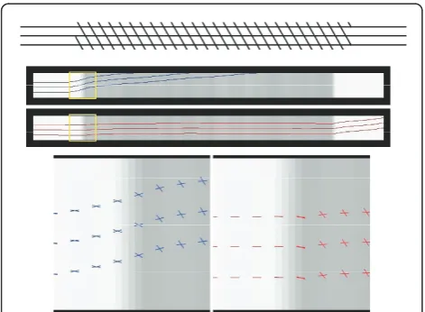
Since the algorithm depends on previous estimations, it is not enough to inspect individual voxels for testing. We construct a 2D field with crossings which the fiber has to navigate through. Figure 1a depicts a schematic of one such field with a 60° crossing. The fibers start on the left in a region with only one true fiber population present, and they try to find their way to the right side. In the middle the fibers encounter a region with cross-ing fibers at a fixed angle. Figure 1b shows the resultcross-ing fibers. In blue we present the simpler model and in red our new full model. The simpler model drifts off shortly after entering the crossing region while our full model maintains a straight path for longer. Outside the cross-ing region, where only one fiber exists, the second com-ponent is aligned with the first. The filter begins estimating a single-tensor until it hits the crossing region where the two components start to point in dif-ferent directions. After the crossing both components will realign again. We generated a set of similar fields for crossings angles of [0°, 5°, ..., 90°].

In Figure 1c we take a closer look at several points along the fibers as they enter the crossing region (the close-up area is marked with a yellow frame in Figure 1b). At every fiber point the principal diffusion direc-tions of both tensors are shown. Again the simpler model is in blue and the full one in red. The principal diffusion directions adapt stepwise, until they are aligned 60° angle in the crossing region. Our full model adapts quicker than the simple model.

3.2 Measurements

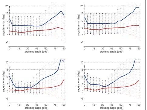
Having verified the underlying behavior, we then began a more comprehensive evaluation. We measured the fol-lowing three different statistics: the average angular error in the non-crossing regions, the average angular error in the crossing region, and the average absolute FA error. With angular error we mean the difference in angle between the principal diffusion directions of the tensors. The estimated values of each fiber point in a certain region (crossing or non-crossing) are compared to the ground truth, the difference is calculated, and the average is taken. The FA error is calculated over both regions at once.

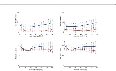
Figure 2 shows the angular error in the non-crossing regions, Figure 3 depicts the angular error in the cross-ing region and Figure 4 displays the absolute FA error. Each graph plots the crossing angle, from 0° to 90°, ver-sus the error. As mentioned we ran every experiment for two different noise levels and forb = 1000 s mm-2 and b= 3000 s mm-2. We seeded from 18 different vox-els in each test scenario, and also, our crossing region is quite large as you can see in Figure 1. This guarantees a fair number of used tensors for averaging. In each graph the trendlines indicate the mean error while the bars indicate the standard deviation.

The graphs for the angular errors show that our new full model generally performs better. In the non-crossing region our model is more stable, especially for the cases with higher crossing angles of 60°-90°. For these angles the simpler model’s error raises quickly while our full model is almost constant. In the crossing region the full model performs better for lower angles 0°-45°. Working with different b-values or with a different noise levels does not significantly change the errors. The absolute FA error is lower and yields a lower variance with our new full tensor algorithm (see Figure 4). This is the expected result of having independent second and third eigenvalues. In the simpler model the second and third eigenvalues have to be identical, which makes it more difficult to match the signal.

3.3 In vivo tractography

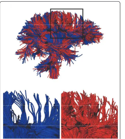
We tested our approach also on a real human brain scan which was weighted with 51 gradients directions. Figure 1 Synthetic tractography experiment testing the

The diffusion-weighted images have a voxel size of

1.66 × 1.66 × 1.7 mm2 and b = 900 s mm-2. Figure 5

shows the results from a tractography started in the right Thalamus of the human brain. The blue fibers were obtained with the simpler fiber model whereas the red fibers were traced with our new full model. At a first glance both methods seem similar but the sepa-rated close-ups in Figure 5b, c show that our approach finds fibers in certain areas where the simpler model stops.

4 Conclusions

We used the tractography framework of Malcolm et al. [43,44] which is built on an unscented Kalman filter and extended the used fiber model. By changing the fiber model and allowing it to have three different,

independent eigenvalues, the tractography procedure was improved and the angular and FA errors were mini-mized. By representing the orientation of the diffusion ellipsoid with Euler angles, the Kalman filter’s state only contains one variable more per tensor than the simpler model. The small increase in calculation time due to this additional variable is negligible. We confirm that using a causal filter for tractography performs much better than independent alternatives. We believe that exploring more alternative fiber models and plugging them into the filtering framework will provide new insights into neural pathways and that they, ultimately, will enhance non-invasive diagnosis of human brains. Furthermore, exploring filtering techniques other than the unscented Kalman filter might yield promising results.

Figure 3These graphs depict the average angular error between the principal diffusion directions of all tensors and the ground truth in crossing region. The simpler model_’s values are displayed in blue while our new full model is in red. Our full model yields a smaller error.a Angular error in crossing region with low noise on the left and high noise on the right,b= 1000 s mm-2_{.bAngular error in crossing region} with low noise on the left, and high noise on the right,b= 3000 s mm-2_.

Author details

1_{Computer Vision Laboratory, ETH Zürich, 8092 Zürich, Switzerland} 2

Psychiatry Neuroimaging Laboratory, Harvard Medical School, Boston, MA, USA3_{Laboratory of Mathematics in Imaging, Harvard Medical School,} Boston, MA, USA

Competing interests

The authors declare that they have no competing interests.

Received: 1 December 2010 Accepted: 27 September 2011 Published: 27 September 2011

References

1. DC Alexander, G Barker, S Arridge, Detection and modeling of non-Gaussian apparent diffusion coefficient profiles in human brain data. Magn Reson Med.48, 331–340 (2002). doi:10.1002/mrm.10209

2. L Frank, Characterization of anisotropy in high angular resolution diffusion-weighted MRI. Magn Reson Med.47, 1083–1099 (2002). doi:10.1002/ mrm.10156

3. A Alexander, K Hasan, J Tsuruda, D Parker, Analysis of partial volume effects in diffusion-tensor MRI. Magn Reson Med.45, 770_–780 (2001). doi:10.1002/ mrm.1105

4. D Tuch, T Reese, M Wiegell, N Makris, J Belliveau, V Wedeen, High angular resolution diffusion imaging reveals intravoxel white matter fiber heterogeneity. Magn Reson Med.48, 577–582 (2002). doi:10.1002/ mrm.10268

5. G Parker, DC Alexander, Probabilistic anatomical connectivity derived from the microscopic persistent angular structure of cerebral tissue. Phil Trans R Soc B.360, 893–902 (2005). doi:10.1098/rstb.2005.1639

6. B Kreher, J Schneider, I Mader, E Martin, J Hennig, K Il_’yasov, Multi-tensor approach for analysis and tracking of complex fiber configurations. Magn Reson Med.54, 1216_–1225 (2005). doi:10.1002/mrm.20670

7. S Peled, O Friman, F Jolesz, CF Westin, Geometrically constrained two-tensor model for crossing tracts in DWI. Magn Reson Med.24(9), 1263–1270 (2006)

8. M Hlawitschka, G Scheuermann, HOT-lines: tracking lines in higher order tensor fields, inVisualization, 27–34 (2005)

9. E Özarslan, T Shepherd, B Vemuri, S Blackband, T Mareci, Resolution of complex tissue microarchitecture using the diffusion orientation transform. NeuroImage.31(3), 1086–1103 (2006). doi:10.1016/j.neuroimage.2006.01.024 10. T McGraw, B Vemuri, B Yezierski, T Mareci, Von Mises-Fisher mixture model

of the diffusion ODF, inInternational Symposium on Biomedical Imaging, 65_–68 (2006)

11. E Kaden, T Knøsche, A Anwander, Parametric spherical deconvolution: inferring anatomical connectivity using diffusion MR imaging. NeuroImage.

37, 474–488 (2007). doi:10.1016/j.neuroimage.2007.05.012

12. Y Rathi, O Michailovich, ME Shenton, S Bouix, Directional functions for orientation distribution estimation. Med Image Anal.13, 432–444 (2009). doi:10.1016/j.media.2009.01.004

13. T Behrens, H Johansen-Berg, S Jbabdi, M Rushworth, M Woolrich, Probabilistic diffusion tractography with multiple fibre orientations: what can we gain?. NeuroImage.34, 144_–155 (2007). doi:10.1016/j. neuroimage.2006.09.018

14. MD King, DG Gadian, CA Clark, A random effects modelling approach to the crossing-fibre problem in tractography. NeuroImage.44, 753–768 (2009). doi:10.1016/j.neuroimage.2008.09.058

15. D Tuch, Q-ball imaging. Magn Reson Med.52, 1358–1372 (2004). doi:10.1002/mrm.20279

16. A Anderson, Measurement of fiber orientation distributions using high angular resolution diffusion imaging. Magn Reson Med.54(5), 1194–1206 (2005). doi:10.1002/mrm.20667

17. C Hess, P Mukherjee, E Han, D Xu, D Vigneron, Q-ball reconstruction of multimodal fiber orientations using the spherical harmonic basis. Magn Reson Med.56, 104–117 (2006). doi:10.1002/mrm.20931

18. M Descoteaux, E Angelino, S Fitzgibbons, R Deriche, Regularized, fast, and robust analytical Q-ball imaging. Magn Reson Med.58, 497–510 (2007). doi:10.1002/mrm.21277

19. C Poupon, A Roche, J Dubois, JF Mangin, F Poupon, Real-time MR diffusion tensor and Q-ball imaging using Kalman filtering. Med Image Anal.12(5), 527_–534 (2008). doi:10.1016/j.media.2008.06.004

20. B Jian, B Vemuri, A unified computational framework for deconvolution to reconstruct multiple fibers from diffusion weighted MRI. Trans Med Imag.

26(11), 1464–1471 (2007)

21. K Jansons, DC Alexander, Persistent angular structure: new insights from diffusion MRI data. Inverse Probl.19, 1031–1046 (2003). doi:10.1088/0266-5611/19/5/303

22. JD Tournier, F Calamante, D Gadian, A Connelly, Direct estimation of the fiber orientation density function from diffusion-weighted MRI data using spherical deconvolution. NeuroImage.23, 1176_–1185 (2004). doi:10.1016/j. neuroimage.2004.07.037

23. R Kumar, A Barmpoutis, BC Vemuri, PR Carney, TH Mareci, Multi-fiber reconstruction from DW-MRI using a continuous mixture of von Mises-Fisher distributions, inMathematical Methods in Biomedical Image Analysis (MMBIA), 1–8 (2008)

24. DC Alexander, Multiple-fiber reconstruction algorithms for diffusion MRI. Annal NY Acad Sci.1046(1), 113–133 (2005)

25. M Descoteaux, R Deriche, T Knoesche, A Anwander, Deterministic and probabilistic tractography based on complex fiber orientation distributions. Trans Med Imag.28(2), 269–286 (2009)

26. PJ Basser, S Pajevic, C Pierpaoli, J Duda, A Aldroubi: in vivo fiber tractography using DT-MRI data. Magn Reson Med.44, 625–632 (2000). doi:10.1002/1522-2594(200010)44:43.0.CO;2-O

27. P Hagmann, T Reese, WY Tseng, R Meuli, JP Thiran, VJ Wedeen, Diffusion spectrum imaging tractography in complex cerebral white matter: an investigation of the centrum semiovale, inInternational Symposium on Magnetic Resonance in Medicine (ISMRM), 623 (2004)

28. W Guo, Q Zeng, Y Chen, Y Liu, Using multiple tensor deflection to reconstruct white matter fiber traces with branching, inInternational Symposium on Biomedical Imaging, 69–72 (2006)

29. C Gössl, L Fahrmeir, BP utz, L Auer, D Auer, Fiber tracking from DTI using linear state space models: detectability of the pyramidal tract. NeuroImage.

16, 378_–388 (2002). doi:10.1006/nimg.2002.1055

30. M Björnemo, A Brun, R Kikinis, CF Westin, Regularized stochastic white matter tractography using diffusion tensor MRI, inMedical Image Computing and Computer Assisted Intervention (MICCAI), 435–442 (2002)

31. F Zhang, E Hancock, C Goodlett, G Gerig, Probabilistic white matter fiber tracking using particle filtering and von Mises-Fisher sampling. Med Image Anal.13, 5–18 (2009). doi:10.1016/j.media.2008.05.001

32. L Zhukov, A Barr, Oriented tensor reconstruction: tracing neural pathways from diffusion tensor MRI, inVisualization, 387–394 (2002)

33. G Parker, DC Alexander, Probabilistic Monte Carlo based mapping of cerebral connections utilizing whole-brain crossing fiber information, in Information Processing in Medical Imaging (IPMI), 684_–696 (2003) 34. T Hosey, R Ansorge, Inference of multiple fiber orientations in high angular

resolution diffusion imaging. Magn Reson Med.54, 1480–1489 (2005). doi:10.1002/mrm.20723

35. Y Iturria-Medina, EJ Canales-Rodríguez, L Melie-García, PA Valdés-Hernández, E Mart_ńez-Montes, Y Alemán-Gómez, JM Sánchez-Bornot, Characterizing brain anatomical connections using diffusion weighted MRI and graph theory. NeuroImage.36, 645_–660 (2007). doi:10.1016/j.

neuroimage.2007.02.012

36. P Fillard, C Poupon, JF Mangin, A novel global tractography algorithm based on an adaptive spin glass model, inMedical Image Computing and Computer Assisted Intervention (MICCAI), 927_–934 (2009)

37. S Jbabdi, M Woolrich, J Andersson, T Behrens, A bayesian framework for global tractography. NeuroImage.37, 116–129 (2007). doi:10.1016/j. neuroimage.2007.04.039

38. B Kreher, I Madeer, V Kiselev, Gibbs tracking: a novel approach for the reconstruction of neuronal pathways. Magn Reson Med.60, 953_–963 (2008). doi:10.1002/mrm.21749

39. W Zhan, Y Yang, How accurately can the diffusion profiles indicate multiple fiber orientations? A study on general fiber crossings in diffusion MRI. J Magn Reson.183, 193_–202 (2006). doi:10.1016/j.jmr.2006.08.005

40. K Seunarine, P Cook, M Hall, K Embleton, G Parker, DC Alexander, Exploiting peak anisotropy for tracking through complex structures, inMathematical Methods in Biomedical Image Analysis (MMBIA), 1–8 (2007)

41. B Jian, B Vemuri, E Özarslan, PR Carney, TH Mareci, A novel tensor distribution model for the diffusion -weighted MR signal. NeuroImage.

37(1), 164–176 (2007). doi:10.1016/j.neuroimage.2007.03.074 42. T Schultz, H Seidel, Estimating crossing fibers: a tensor decomposition

approach. Trans Vis Comput Graph.14(6), 1635–1642 (2008)

43. JG Malcolm, ME Shenton, Y Rathi, Neural tractography using an unscented kalman filter. Inf Process Med Imaging (IPMI).21, 126–138 (2009) 44. JG Malcolm, ME Shenton, Y Rathi, Filtered multi-tensor tractography. IEEE

Trans Med Imaging.29, 1664–1675 (2010)

45. CG Koay, LC Chang, C Pierpaoli, PJ Basser, Error propagation framework for diffusion tensor imaging via diffusion tensor representations. IEEE Trans Med Imaging.26(8), 1017–1034 (2007)

46. S Julier, J Uhlmann, Unscented filtering and nonlinear estimation. IEEE.

92(3), 401–422 (2004). doi:10.1109/JPROC.2003.823141

47. R van der Merwe, E Wan, Sigma-point Kalman filters for probabilistic inference in dynamic state-space models, inWorkshop on Advances in Machine Learning(2003)

48. Y Rathi, JG Malcolm, S Bouix, CF Westin, ME Shenton, False positive detection using filtered tractography, inInternational Symposium on Magnetic Resonance in Medicine (ISMRM)(2010)

49. PJ Basser, C Pierpaoli, Toward a quantitative assessment of diffusion anisotropy. Magn Reson Med.36(6), 893_–906 (1996). doi:10.1002/ mrm.1910360612

doi:10.1186/1687-6180-2011-77

Cite this article as:Lienhardet al.:A full bi-tensor neural tractography algorithm using the unscented Kalman filter.EURASIP Journal on Advances in Signal Processing20112011:77.

Submit your manuscript to a

journal and benefi t from:

7 Convenient online submission

7 Rigorous peer review

7 Immediate publication on acceptance

7 Open access: articles freely available online

7 High visibility within the fi eld

7 Retaining the copyright to your article