New Methods for Reliability Evaluation and Enhancement of Power Systems

(1)

New Methods for Reliability

Evaluation and Enhancement of

Power Systems

By

Rahamathulla Mohammad

Thesis submitted to the College of Engineering and Science

Victoria University Melbourne, Australia

In-fulfilment of the requirements for the degree of

DOCTOR OF PHILOSOPHY

In

Electrical Engineering

Prof. Akhtar Kalam

Principal Supervisor

And

Dr. Suprasad Amari

External Industry Supervisor

(2)

Declaration

“I, Rahamathulla Mohammad, declare that the PhD thesis entitled ‘New Methods for Reliability Evaluation and Enhancement of Power Systems’ is no more than 100,000 words in length including quotes and exclusive of tables, figures, appendices, bibliography, references and footnotes. This thesis contains no material that has been submitted previously, in whole or in part, for the award of any other academic degree or diploma. Except where otherwise indicated, this thesis is my own work”.

(3)

List of Figures

Figure 2.1: Bath tub shaped hazard rate function graph…… 15

Figure 2.2: Components of Reliability and Cost……… 27

Figure 3.1 – Graphical Representation of Sequence (1)……… 37

Figure 3.2 – Graphical Representation of Sequence (2)……… 38

Figure 4.1: The elements of Geothermal Power Plant……… 47

Figure 4.2: Markov Chain for k-out-of-n Systems with Active Redundancy.52 Figure 4.3: Markov Chain for k-out-of-n System with Warm Standby Redundancy……… 52

Figure 5.1: Non-homogeneous Markov process for Identical components case. 66 Figure 5.2: Non-homogeneous Markov process after substituting αi ……… 77

Figure 5.3: System failure process using non-homogeneous Markov chain 68 Figure 5.4:Non-Homogeneous Markov Chain ……… 68

Figure 5.5: Homogeneous Markov Chain ……… 69

Figure 7.1: Typical 400KV substation, the control room and EWS in action.95 Figure 7.2: Wiring diagram for digital inputs ……… 95

Figure 7.3: EWS Typical Layout showing RS-232 AND RS-485 ……… 96

Figure 7.4: A solution to improve the reliability of Railway Signaling and Telecommunications. ………. 99

Figure 7.5: Existing M2M setup ……… 105

(9)

(10)

List of Tables

(11)

List of Acronyms

AFTM Accelerated Failure Time Model CB Circuit Breaker

CE Cumulative Exposure Model CPU Central Processing Unit EHV Extra High Voltage EWS Early Warning System FTS Fault-Tolerant System

GMSSkn Generalized Multi-State k-out-of-n System HVDC High Voltage Direct Current

i.i.d Independent and Identical Distributed LSS Load Sharing System

(12)

PHM Proportional Hazards Model PMS Phased-Mission System RAPS Remote Area Power Supplies rms Root Mean Squared

SCADA Supervisory Control And Data Acquisition SS Sub-system

S&T Signalling and Telecommunication TFR Tampered Failure Rate

(13)

Nomenclature

t Mission time

n Number of components in system

k Minimum number of working components required for system success

pj Probability of having exactly i component failures in a [logical] location

Pj Probability of having exactly i component failures in system

Qj Probability of failure sequence i  Parameter of Rayleigh distribution

f(t) Probability density function (pdf)

F(t) Cumulative distribution function (cdf)

R(t) Component reliability

psw Switch success probability on demand

RSys(t) System reliability

x!! Double factorial function; If x is even: x!! = x(x-2)…3.1 FN(t) Cdf of Nakagami distribution

I(a,x) Regulated gamma function

M Number of phases

Duration of phase j; j = 1,…,M;

(14)

S Total number of sub-systems

n Number of components in a given sub-system; It can vary for each sub-system.

kj Minimum number of working components required for a given sub-system

in phase j;

It can vary for each sub-system.

mj Defined as:

Minimum number of failed components required for a given sub-system to fail in phase j;

λoj Failure rate of an operating component in phase j

λdj Failure rate of a dormant component in phase j

dj Defined as: dj = λdj / λoj , dormancy factor of a component in phase j.

Defined as:

Rl Reliability of sub-system l

RPMS Mission reliability of PMS

n Number of components in the system

k Minimum number of components required for successful operation

zi Load on each component when i components failed;

Baseline failure rate of PHM

(15)

Initial probability state vector

R(t) System reliability

M Number of phases

Duration of phase j; j = 1,…,M;

T Mission time:

N Total number of sub-systems

n Number of components in a given sub-system;

It can vary for each sub-system. Hence, n = nl for sub-system l.

kj Minimum number of working components required for a given sub-system

in phase j;

It can vary for each sub-system. Hence, kj = kli for sub-system l inphase j.

mj Defined as:

LT Total load on a sub-system in a given phase;

It can vary for each sub-system. Hence, LT = LT(l,j) for sub-system l in

phase j.

(L) Failure rate function in load L;

(L) =l(L) for the components in sub-system l

i Failure rate of a component when there are i failures in the sub-system;

It can vary for each phase and sub-system. Hence, i = i(l,j) for

sub-system l inphase j.

Si State-i of a sub-system; it is equivalent to the sub-system state with i

failures.

(16)

It can vary for each phase and sub-system. Hence, i = i(l,j) for

Pa,i Conditional probability that a given sub-system is in state-i at the end of a

phase given that was in state-a at the beginning of the phase;

It can vary for each phase and sub-system. Hence, Pa,i = Pa,i(j,l) for

 System structure function

Rl Mission reliability of sub-system l

(17)

ABSTRACT

Modern Power systems are smart, interconnected, interdependent, load sharing and phased mission systems. Reliability of such complex power systems is very important in design, planning, installation and maintenance to provide electrical energy as economical as possible with an acceptable degree of reliability. In this thesis four new methods for reliability evaluation and enhancement of power systems are presented and further an innovative cost effect cloud service based smart early warning system using machine to machine (M2M) technology to improve the reliability of power systems is presented.

(18)

need for one-dimensional convolution integrals using approximate closed-form expressions for computing the distribution of sum of Rayleigh distributed random variables. This new method shows that all steps involved in evaluating the reliability of k-out-of-n cold standby system with components having Rayleigh operational failure time distributions are simple and straightforward. The proposed method and its computational efficiency and accuracy are illustrated using a numerical example.

With the development of technology, sensor networks, and non-conventional power generators, became more and more complex, and their missions become more and more diversified. Further, many real world power systems operate in phased-missions where the system requirements and success criteria vary over consecutive time periods, known as phases. For mission success, all phases must be completed without failure. In order to ensure accomplishing missions successfully, many sub-systems adopt redundancy techniques to improve the mission reliability. Particularly, redundancy is an effective method to improve the reliability of mission critical power systems. Hence, there is a great need for accurate and efficient reliability evaluation of phased mission systems with phase dependent redundancy configurations and requirements.

(19)

vary with the phases. Similarly, the configuration of each sub-system can vary with the phases. The proposed algorithm is developed based on: (1) a modularization technique, (2) an easily computable closed-form expressions for conditional reliability of warm standby sub-system with phased dependent success criteria, and (3) a recursive formula for accounting the dependencies of sub-systems across the phases. As cold and hot standby configurations are special cases of warm standby configuration, the proposed method is also applicable for analysing the phased mission systems with cold and hot standby redundancies. The reliability evaluation algorithm is illustrated using an example of fault tolerant power system.

In the thesis a third new model for load-sharing systems using k-out-of-n

(20)

is the product of both a baseline hazard rate, which can be a function of time ‘t’, and a multiplicative factor which is a function of the current load on the component. In addition, the load-sharing model also considers the switchover failures at the time of load redistribution. This research shows that the model can be described using a homogeneous Markov chain. Therefore, for the non-identical component case, the system reliability can be evaluated using well established methods for non-homogeneous Markov chains. In addition, when all components are identical, this thesis provides a closed-form expression for the system reliability even when the underlying baseline failure time distribution is non-exponential. The method is demonstrated using a numerical example with components following Weibull baseline failure time distribution. The numerical results from non-homogeneous Markov chains, closed-form expressions, and Monte Carlo simulation are compared.

(21)

Finally, the development of a cost-effective, cloud service based smart early warning system for improving the reliability of power systems using M2M technology is presented.

(22)

ACKNOWLEDGEMENT

I would like to express my heartfelt gratitude and sincere thanks to my principal supervisor, Prof. Akhtar Kalam for his kind guidance and supervision throughout the course of my research.

I would like to thank my external supervisor Dr. Suprasad Amari for his kind guidance and supervision. I could not have completed this thesis without his guidance, invaluable support, and constant encouragement from US.

I would like to express my sincere gratitude to “Arka Industrial Monitoring Systems Pvt., Ltd., Hyderabad, India” for assisting me in the development of hardware and software required for my project. I am very thankful to the staff for allowing me to collect data from the field. Without their support in collecting data from the field it is not possible to complete this research project. My special thanks to Ravikiran Akella product design engineer, Karimullah Mohammad Power Engineer and Arun Sapkal delivery manager for their support during my research, guiding me in right direction and allowing me to visit their R & D facilities.

I must thank Dr. Zaheer Paracha for his motivation to start my research in power engineering.

My special thanks to my research colleague Dr.Kannan.J for supporting during our break though research discussions, experiments in power lab, writing research papers and valuable support in attending international conference in India along with my supervisor.

(23)

(24)

CHAPTER 1

1 THESIS OVER VIEW

1.1 Background

(The content of this Chapter has been presented at Reliability and Maintainability Symposium (RAMS) 2012 & 2013 conferences USA)

Reliability relates to the ability of a system to perform its intended function, in a qualitative sense. Planners and designers are always concerned with reliability. When qualitatively defined, reliability becomes a parameter that can be treated off with other parameters like cost. Necessity of qualitative reliability is an ever increasing complexity of systems, evaluations of alternate designs, cost competitiveness and cost benefit trade off. Due to fast extension of liberalization of power systems, innovation in technology, due to very short product development times, tightened budgets not giving enough time to do the reliability tests, there is no failure data occurs during those tests. In electrical engineering, Smart Grid connected power systems are facing above Reliability challenges. Therefore there is a big need to develop new methods for Reliability evaluations and enhancement of power systems based on not only an experimental data but also on technological and physical information available to the engineers. Overvoltage, Loads, Short-Circuits and weather conditions relates to wear and stress acting on the components/devices/equipment in power systems. A typical model of aging can be expressed mathematically by time behaviour of its hazard rate

(25)

function. Most electronic components are scarcely affected by aging and their failure is mainly accidental, so that a constant hazard rate function could be reasonably expressed. This leads to the adaptation of an exponential model in power systems, even in the absence of many data to support it on a statistical basis. Selection or correct identification of suitable probabilistic model for power system component reliability in the field of high reliability devices and large mission times should be better supported by probabilistic information that leads to reasonable modelling in medium voltage and high voltage components.

(26)

great need to find new methods for reliability evaluation of load sharing system. The weakest part of a power device is its insulation, the predominant stress acting on insulation in service does commonly arise from the electric field associated with electric stress (Voltage) and the temperature associated with Joule losses in conducting elements plus dielectric losses in the insulation. Therefore, in general the maximum stress applied to a power system is maximum temperature and electric field in the insulation. In this framework, the life of power system subjected to load cycles is assumed here to end when its insulation fails because of the degradation caused by the maximum stress, that act all over its life as a consequence of a fixed stepwise constant daily load cycle.

1.2 Significance of the project

The significance of this project is that it presents the work towards the Reliability evaluation issues and solutions of power systems such as cold standby sub-system with components having linearly increasing hazard rates, warm standby sub-systems, load-sharing power systems, phased mission systems with load-sharing components subjected to switch failures in power systems, and development of a cost effective cloud service based, smart grid integration capable system to improve the reliability of power systems using M2M technology.

1.3 Scope and Objectives of the Project

(27)

1. By using the concepts of counting processes, an efficient approximate method to evaluate the reliability of k-out-of-n cold standby systems is proposed. This proposed method considers Rayleigh distributions for component life times and the effects of switch failures on system reliability.

2. A new method for reliability analysis of phased-mission systems with warm standby sub-systems is presented.

3. Reliability of load-sharing systems subject to proportional hazards model is presented. This method is demonstrated using a numerical example with components following Weibull baseline failure time distribution. The numerical results from non-homogeneous Markov chains, closed-form expressions, and Monte Carlo simulation are compared.

4. An efficient recursive algorithm for reliability evaluation of phased mission systems with load-sharing components subjected to switch failure is proposed.

(28)

1.4 Thesis Outline

This thesis comprises eight Chapters. Organization of the remaining seven Chapters is presented below:

Chapter 2 presents number of past efforts related to the current work. It presents literature review of past attempts in the area of Power System Reliability.

In Chapter 3, by using the concepts of counting processes, an efficient approximate method to evaluate the reliability of k-out-of-n cold standby systems is proposed. This proposed method considers Rayleigh distributions for component life times and the effects of switch failures on system reliability. The main advantage of this counting process-based method is that it reduces a complex problem involving multiple integrals into an equivalent simple problem involving one-dimensional convolution integrals. This research further eliminate the need for one-dimensional convolution integrals using approximate closed-form expressions for computing the distribution of sum of Rayleigh distributed random variables. Hence, this research shows that all steps involved in evaluating the reliability of k-out-of-n cold standby system with components having Rayleigh operational failure time distributions are simple and straightforward. This Chapter illustrates the proposed method and its computational efficiency and accuracy using a numerical example.

(29)

In Chapter 5, the load-dependent time-varying failure rate of a component is expressed using Cox’s proportional hazards model (PHM). According to the PHM the effects of the load is multiplicative in nature. In other words, the hazard (failure) rate of a component is the product of both a baseline hazard rate, which can be a function of time ‘t’, and a multiplicative factor which is function of the current load on the component. In addition, the load-sharing model also considers the switchover failures at the time of load redistribution. Here first it is shown that the model can be described using a non-homogeneous Markov chain. Therefore, for the non-identical component case, the system reliability can be evaluated using the established methods for non-homogeneous Markov chains. In addition, when all components are identical, this Chapter provides a closed-form expression for the system reliability even when the underlying baseline failure time distribution is non-exponential. The method is demonstrated using a numerical example with components following Weibull baseline failure time distribution. The numerical results from non-homogeneous Markov chains, closed-form expressions, and Monte Carlo simulation are compared.

(30)

In Chapter 7, a remote fault detection and identification system, for generation, transmission and distribution (GTD) system, for both renewable and non-renewable sources to minimize failures and their effects using innovative hardware and software system integration with M2M technology and cloud computing is presented.

Chapter 8 summarizes the work as well as presents the future directions of research.

1.5 List of Publications

The following are publications related to this work:

1. Mohammad, R.; Kalam, A.; Amari, S.V., "Reliability evaluation of phased-mission systems

with load-sharing components," Reliability and Maintainability Symposium (RAMS), 2012 Proceedings- Annual , vol., no., pp.1,6, 23-26 Jan. 2012. doi: 0.1109/RAMS.2012.6175468 2. Mohammad R, Kannan J, Kalam A and Zayegh A “ Reliability Analysis of T-1000 1.2 kW

PEMFC Power Generation System with Load-Sharing using MATLAB” International

Conference in Renewable Energy Utilization, ICREU 2012, organised by Oklahoma State

University, Stillwater USA and CIT India.

3. Kannan J , Mohammad R, Akhtar Kalam, Aladin Zayegh “ Reliability Analysis of a

Wind/Solar 4kW Micro-Generation System with Load Sharing using MATLAB”

International Conference in Renewable Energy Utilization, ICREU 2012, organised by

Oklahoma State University, Stillwater USA and CIT India.

4. Mohammad R, Kalam A, Amari V. Suprasad “Reliability of k-out-of-n Cold Standby Systems with Rayleigh Distributions” Proceeding of 18th ISSAT International conference on Reliability and Quality Design. July, 2012, Boston USA, pp 188-193

5. Mohammad, R.; Kalam, A.; Akella, R., "A cost-effective early warning system for

(31)

(RAMS), 2013 Proceedings - Annual , vol., no., pp.1,6, 28-31 Jan. 2013 doi: 10.1109/RAMS.2013.6517731.

6. Mohammad, R.; Kalam, A.; Amari, S.V., "Reliability of load-sharing systems subject to

proportional hazards model," Reliability and Maintainability Symposium (RAMS), 2013 Proceedings - Annual , vol., no., pp.1,5, 28-31 Jan. 2013 doi: 10.1109/RAMS.2013.6517708 7. Mohammad, R.; Kalam, A.; Amari, S.V., "Reliability of phased mission systems with warm

standby sub-systems," Reliability and Maintainability Symposium (RAMS), 2013 Proceedings - Annual , vol., no., pp.1,5, 28-31 Jan. 2013 doi: 10.1109/RAMS.2013.6517753.

8. Mohammad, R.; Kalam, A., "Development of a Cost-Effective, Smart Early Warning

System for Improving the Reliability of Electrical Substations”, Submitted for a journal

publication

9. Mohammad, R.; Kalam, A.; Amari, S.V., "Development of a Cost-Effective, Early Warning

System for Improving the Reliability of standalone renewable power system by using M2M

Technology”, submitted for a journal publication.

10. Mohammad, R.; Kalam, A., ”Reliability Evaluation of Phased Mission Systems with

(32)

CHAPTER 2 LITERATURE REVIEW

2.1 Literature Review

2

(Some of the content in this Chapter has been presented in RAMS conference 2011)

The purpose of this Chapter is to provide the necessary background required for understanding the Reliability of Power Systems. It also highlights the concepts that related to recent developments in this field. This Chapter begins by presenting the need for this research and some of past research efforts in the field of Power systems Reliability.

Recent blackouts in Victoria, Queensland, New South Wales and in other parts of the Australia due to bush fires, floods and other natural disasters including Fukushima nuclear disaster have, however, focused attention on the need for an investigation and evaluations of Electrical Power Systems. Power system is a complex system, has numerous facilities and structures, systems and sub-systems, components and equipment, and has a complex communication among all those. The basic function of a power system is to supply energy as economically as possible and with a reasonable degree of continuity and quality its intended system. Power system reliability can be assessed based on system configuration, aging, component reliability and delivery of power to the load. Due to its complexity, power system has many issues in the field of power systems reliability.

Over the last 10 years, Victoria has suffered major blackouts each year. In February 2005, storms kept 410,000 Victorians off the power supply. In January 2006, high temperature and

(33)

storms caused 618000, supply interruptions. In 2007, a bush fire forced rolling power shut down across Victoria. In April 2008, storms took 420000, Victorians off supply for days. In January 2009, break downs in distribution and transmission and problems with the bass link interconnect caused power supply loss more than 500,000 Victorians [5].

Reliability is one of the most important criteria, which must be taken into consideration during planning and operation phases of a power system. Electric power sector almost all over the world is undergoing considerable changes in regard to structure, operation and regulation which includes Smart Grids, Embedded Generation/Micro Generation (Roof top PVs, Wind forms, Geothermal and Gas-fired power stations), However, from the reliability point of view in this “new era”, methods, algorithms and computer software capable of assessing at least the adequacy of systems much larger than in the past are needed [6,7]. To minimise the possibility of future blackouts, requires implementation of reliability policies that emphasize four factors essential to meeting the requirements of the new standards:

1. Continued development of sufficient electric generation resources, transmission delivery infrastructure, and demand response programs to reliably meet forecasted future electricity demands.

(34)

both planned and unforeseen changes to the system.

Many recommendations have already been addressed, as indicated in the final report of the task force on implementing recommendations in [8], but work remains in several areas that are more difficult to address. These include developing new or revised standards or guidelines in protective relay system design, application, maintenance, and testing; under voltage load shedding systems; and voltage and reactive planning and operation; as well as developing and implementing improved real-time system visualization tools for systems operators, including measurement systems; etc. [8]

The Australian Energy Market Operation (AEMO) is responsible for planning and directing the augmentation of the shared transmission networks. AEMO applies a probabilistic approach to planning the Victorian shared transmission network. Under that approach, investment only proceeds when the expected benefit exceeds the cost. The probabilistic approach involves the occurrence of plant outages occurring within the peak load season and weighting the cost of such an occurrences by its probability [9].

(35)

Governments, AEMO and Private Investors are working closely in building wind forms, solar power generation stations, Geothermal power plants and other micro-generation plants, to connect to the electricity declared shared network, which creates greater need for the reliability analysis of these systems. The current research effort is related to the need to know the reliability of this system accurately, efficiently and fast.

(36)

conducted with severe time constraints and no failure data occurs during these tests. In particular smart grid connected power systems are facing above reliability challenges. Therefore there is a need to develop new methods for reliability evaluation and enhancement of power systems based on not only on experimental data but also on technological and physical information related to wear and stress such as over voltages, loads and short circuits acting on the components, devices and by time behaviour of their hazard rate function. Most electronic components in power systems are affected by aging, their failure is mainly accidental, so aging failures in power systems is a big concern and a driving factor in system planning in many power systems. More and more power system components are reaching their end of life period; therefore ageing failure must be included in power system reliability evaluation.

Electrical systems failure depends on factors such as loads, redundancies and configurations. There are different mathematical models to evaluate the reliability of existing power systems but non-of the existing models provide accurate reliability. The aim of this research is to develop advanced algorithms which are computationally efficient, provide practically and accurately evaluate the reliability of the existing and future Smart- Grid applications of Victorian power systems.

(37)

2.2 Reliability and Hazard Functions

Reliability is the probability that a product will operate or service will be provided properly for a specified period of time under the design operating condition without failure. Reliability of a system is analysed based on the reliability analysis of components of that particular system on the basis of failure data from devices in-service. Performing a direct reliability analysis requires that the most adequate probability distribution for the reliability analysis to be chosen from a family of commonly employed distributions for such components is selected on the basis of a combination of all these aspects. The most adopted reliability models for electrical components of any power system are Gamma, Normal, Lognormal and Weibull. Recently Inverse Gaussian distribution, the Inverse Weibull distribution, the Birnbaum-Saunders distribution, the Log-logistic distribution and more are significantly used for electrical components reliability in power systems.

Hazard function h(t) is the conditional probability of failure in time interval ‘t’ to (t+dt), given that there was no failure at time ‘t’ divided by the length of the time interval dt.

(2.1)

Where f(t) is probability density function and R(t) is reliability function.

The cumulative hazard function H(t) is the conditional probability of failure in the interval 0 to ‘t’.

If the total number of failures during the time interval 0 to t.

(38)

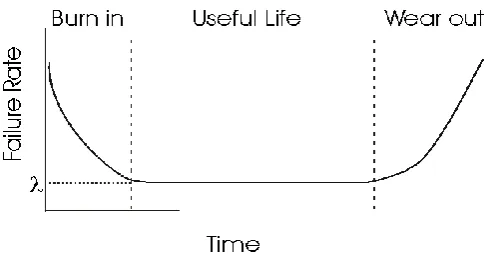
Hazard function is also referred as hazard rate or instantaneous failure rate in reliability theory. It is very important for power system design engineers, repair and maintenance people. Hazard rate is a function of time and it is a bathtub-shaped function shown figure 2.1:

Figure 2.1: Bath tub shaped hazard rate function graph The life of components follow three major periods:

1. Infant mortality period or decreasing failure rate period

(2.3)

2. Useful life period or constant failure rate period

(2.4)

3. Wear-out period or increasing failure rate period

(39)

systems such as rotating shafts, valves and cams- exhibits linearly increasing hazards rate due to wear out, whereas components such as sprigs and elastomeric mounts exhibit linearly increasing hazard rate due to deterioration. Relays in power systems also exhibit linearly increasing hazard rate. Most power system components (both mechanical and electrical) exhibit decreasing hazard rates during their early lives.

When Hazard rate function [h(t)] cannot be represented linearly with time then Weibull model is used where

( ) (2.5)

where are life and share parameters of the distribution.

When components or products experience two or more failure modes then hazard rate is described by Mixed Weibull model. If the hazard function is initially constant and then begins to increase rapidly with time then exponential model is used, where

_(2.6)

Where b is constant and represents the increase in failure rate per unit time. Most of the mechanical components in power systems, subjected to repeated cyclic loads exhibit normal hazard rates. But there is no closed form expression for the reliability or hazard rate functions. The CDF of the life of a component is represented by:

[ ] ∫

√ [ (

₎ _]

(2.7)

And

(40)

Where are mean and the standard deviation of the distribution. Unlike other distributions, the integral of the cumulative distribution cannot be evaluated in a closed form. The pdf for the standard normal distribution is:

√ ( ) (2.9)

Where The CDF is ∫

√ ( )

(2.10)

Therefore, when the failure time of a component is expressed as a normal distributed random variable T, with mean and standard deviation , then the probability the component will fail by time t is given by

( ) ( ) . (2.11)

The right side of this equation can be evaluated using the standard normal distribution. The hazard rate function h(t) of normal distribution is

( ₎

. (2.12)

One of the most widely used probability distribution is describing the life of data resulting from a Semiconductor failure mechanism in power systems is lognormal distribution. It is also used in predicting accelerated life test data. The pdf of lognormal distribution is:

√ [ (

₎ _]

(41)

[ ] [ (2.14) Thus, the hazard rate function is

( ₎

(2.15)

Gamma distribution is another widely used hazard rate function. It has decreasing, constant, or increasing hazard rates. The gamma distribution is suitable for describing the failure time of a component whose failure take place in n stages or the failure time of a system that fails when n independent sub failures have occurred. The gamma distribution is characterised by two parameters: shape parameter and scale parameter . When , the failure rate monotonically decreases from infinity to as time increases from 0 to infinity. When , the failure rate monotonically increases from to infinity, when , the failure rate is constant and equal to .

The pdf of a gamma distribution is

(2.16)

The reliability function

∑ ( )

(2.17)

The hazard rate of the gamma model, when is an integer n is:

( )

∑ ( )

(42)

2.3 Standby Systems

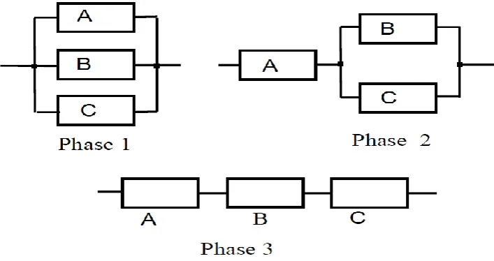
Safety critical power systems including the applications of phased-mission systems use either active or standby redundancy to improve the mission reliability. In general, there are three types of standby configurations, i.e., cold, hot and warm standby configurations. Cold standby implies that the inactive redundant components have a zero failure rate and cannot fail while in standby state. Hot standby implies that the redundant component has the same failure rate as active components while in standby state. Warm standby implies that an inactive component has a failure rate between cold standby and hot standby. Warm standby components are partially powered up when they are in standby mode. Therefore, they have a reduced failure rate in the standby mode. However, they are subject to the regular full failure rate when they are kept in operation to replace the faulty primary components. As compared to hot sub-systems, warm sub-systems do not consume much power when they are in standby mode. As compared to a cold standby system, the warm standby system does not need long initialization and recovery time.

(43)

system with redundant components/sub-system/systems is important to assess whether the power systems meet safety and reliability requirements and to determine the optimal redundancy configurations and other design alternatives [20].

2.4 Reliability of Phased Mission Systems

(44)

but it is often more expensive in computational requirements [39]. This is particularly a concern with the crude Monte Carlo simulation for analysing safety-critical systems, especially those with ultra-high reliabilities often found in nuclear industry.

Therefore, all existing methods for PMS reliability analysis are limited to either small-scale problems (analytical methods) or non-critical systems with moderate reliability requirements (crude Monte Carlo simulation). New methods for reliability evaluation of phased mission systems to overcome the existing issues are investigated in this thesis.

2.5 K-out-of-n Systems

The k-out-of-n system structure has wide range of applications in reliability engineering. It is a common practice to use redundancy techniques to improve the system reliability and availability. A system will be working as long as k components are working in a system out of n components. If ‘k+1’ components fail out of ‘n’ components then the system will fail [8]. For example 1-out-of-4 remote area power system, at least one of the solar panels must be working out of 4 panels for the power system to function.

The reliability of a k-out-of –n system with identical components is evaluated by using binomial distribution.

∑ (₎

∑ (₎ (2.19)

Where p(t), q(t), and f(t) are the reliability, unreliability, failure (hazard) rate, and probability density function (pdf) of each component at time ‘t’.

In [16] several algorithms to compute the reliability of k-out-of-n system with non-identical components are proposed which have computational complexity and requires less memory than other algorithms proposed in other research papers. In [14] efficient reliability evaluation algorithms for binary k-out-of-n system with independent component is provided as:

(45)

Where R(n,k) is the recursive function to evaluate reliability of k-out-of-n system. pn is the

reliability of component n, and qn=1-pn.

The boundary conditions are:

In [20] binary k-out-of-n system has been generalized with binary weighted k-out-of-system, with a recursive equation shown below:

(2.21)

Where R(i,j) is the probability that the system with ‘j’ components can output a total weight of at least ‘i’. The boundary conditions are:

There may be more than two different performance levels in some practical systems such as:

a power generator in a power station can work at full capacity, which is its nominal capacity,

say 100MW, when there are no failures at all. Certain type of failures can cause the generator

to fail completely, while other failures will lead to the generator working at reduced capacity

say 40MW. On the system level, it can be considered that the power generating system

consisting of several power generators. The abilities of the system to meet high power load

demand, normal load demand and lower power load demand can be regarded as different

system states. The reliability evaluation of such system is done through multi-state k-out-of-n

system modelling and evaluation. In [15] the first multi-state k-out-of-n system model is

defined. Here the system state was defined as the state of the kth best component. At any

state j, for the system to be in state j or above, there should be at least k components in state j

or above. That is, the k value is the same with respect to all states. In[16] a generalized

multi-state k-out-of-n:G system model was proposed. In this model there can be different k values

with respect to different states. In [17] an efficient recursive algorithm for reliability

evaluation of generalized multi-state k-out-of-n system with identically and independently

(46)

In [18] another multi-state weighted k-out-of-n model is proposed with more practical

applications. This model has more flexibility in modelling systems involving

weighted-k-out-of-n structure. In [19] Universal Generating Function (UGF) approach is developed to

evaluate multi-state systems. In the binary weighted k-out-of-n system, UGF for the

components is:

_(2.22)

To obtain the UGF of the system based on the individual UGF of the components, the

following composition operator Ω is used:

(2.23) Where

( ) ( )

(2.24)

( )

(2.25)

( ) [∑ ∑

] ∑ ∑

(2.26)

From the above equation system reliability is as shown below for an arbitrary k using an

operator :

∑ ∑ (2.27)

Where in the above equation is:

{

The recursive algorithm for reliability evaluation of the multistate weighted k-out-of-n

systems given for two models. Recursive function for the probability of the system to be in

(47)

system to have sum of useful weights of at least k when one is evaluating the probability for

the system to be in state j or above as

( ) ∑

( ) (2.28) Where

The UGF of each multi-state component is given by:

(2.29) ₍₎

( ) ∑ ( ) (2.30) Where

The UGF for the individual component is as shown below:

(2.31) Where

n: the number of components in the system

M: the highest possible state of each component

: the weight of component I when it is in state j

: Pr{Component i is in state j}

: Pr{Component i is in state below j}, ∑

the minimum total weigh required to ensure that the system is in state j or above.

In [17] an example to illustrate the modelling of power system as a decreasing multi-state

(48)

generator is treated as a component and there are 3 components in this system. Each

generator may be three possible states, 0, 1, and 2. When a generator is state 2, it is capable of

generating 10 MW; in state 1, 2MW; and in state 0, 0MW. The total power output of the

system is equal to the sum of the power output from all three generators. The system may

also be in three different states: 0,1, and 2. When the total output is greater than or equal to

10MW, in state 1; otherwise, in state 0. The reliability of the cluster of power generators in

Smart-Grid can be calculated with the help of formulae shown above. The methods for

analysing and evaluating the reliability of ‘k-out-of-n’ systems shown above are complex. In

this thesis new methods have been proposed. These methods are simple, computationally

(49)

2.6 PHM and Its Significance To

This Research

Modern Power Systems’ management requires the accurate assessment of current and the prediction of future health condition is crucial in the era of Smart-Grid. Suitable mathematical models that are capable of predicting Time-to-Failure (TTF) and the probability of failure in future are very important. The life of power system is influenced by different risk factors called covariates. The basic idea in reliability theory is the failure time of a system and its covariates. These covariates change stochastically, may influence and indicate the failure time of power systems. Until now, a number of statistical models have been developed to estimate the hazard of a system with covariates in reliability field. Most of these models are developed based on the Proportional Hazard Model (PHM) theory which was proposed by cox [51]. This model provides an estimate of the maintenance effect on survival after adjusting for other explanatory variable. It allows the engineers to estimate the failure (hazard) of a component or sub-system or system, given their predictive variables. Cox’s PHM for statistical explanatory variable is expressed as . Where, is the unspecified baseline hazard function which is dependent on time only and without influence of covariates. The positive function term, , is dependent on the effects of different factors, which have multiplicative effect on the baseline hazard function.

The proportionality assumption in PHM is that:

[ ] (2.32)

(50)

systems subjected to PHM. In this thesis the research work undertaken to solve the problem of aging load-sharing systems.

2.7 Reliability and Cost Analysis

Basics

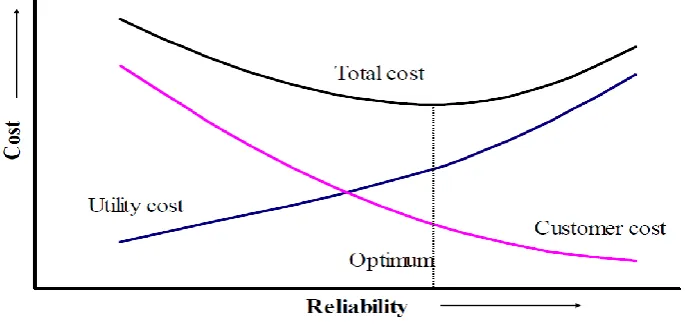
Australian Energy Market Commission stated that by reducing the reliability standards for NSW state electricity distribution network, the government can save up to A$2.5 billion over 15 years and consumers can benefit by getting cost reduction in their electricity bills. The reliability of a system can be improved by installing additional components. The customer interruption costs in these cases will decrease as the capital and operating costs increase. The main objective is to balance the benefits realized from providing higher reliability and the cost of providing it. A major objective of reliability cost assessment is to determine the optimum level of service reliability. This basic concept is shown in figure 2.2. It is shown in the figure that the utility cost increases while the socio-economic customer interruption cost decreases with increase in the level of service reliability. The total cost is the sum of the two curves. The optimum level of reliability occurs at the point of lowest total cost.

(51)

2.8 Conclusions

(52)

CHAPTER 3 RELIABILITY OF K-OUT-OF-N

COLD STANDBY SYSTEMS WITH

RAYLEIGH DISTRIBUTIONS

3

3.1. Introduction

Cold standby redundancy is used as an effective mechanism for improving system reliability [21]. For example, applications of cold standby redundancy can be found in space explosion and satellite systems [22], electrical power systems [23], telecommunication systems [24], textile manufacturing systems [25], and carbon recovery systems [26]. Cold standby redundancy involves the use of redundant components that are shielded from the operational stresses associated with system operation. Without exposure to those stresses, the likelihood of failure is very low, and assumed to be zero, until the component is required to operate as a substitute for a failed component [21]. When a failure does occur, it is necessary to detect the failure and to activate the redundant component. For a non-repairable system, the failure detection and switching must be accomplished by additional system hardware that would not otherwise be required. When switching mechanisms are perfect, standby redundancy can provide higher system reliability compared to active redundancy with analogous system architecture [21, 27]. However, when switching mechanisms are imperfect, cold standby redundancy may not necessarily provide higher system reliability than the corresponding active redundancy system [8]. Therefore, for analysing the reliability of cold

3_{Contents of this Chapter have been presented at 18}th_{ISSAT International conference on Reliability and Quality Design. July, 2012,}

(53)

standby systems, it is important to consider switching failures [21, 27-29].

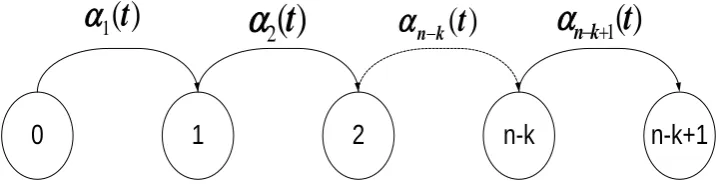
When component failure times follow a non-exponential distribution and the system requires multiple operating components for its success (k > 1), then the successive failures of the k-out-of-n cold standby system do not follow any standard stochastic process [7, 9]. This is because, at any given time during the mission, the system can have multiple working components with different operational times (operational ages). Therefore, to calculate the probability of another failure during the mission, the operational ages of all working components must be considered. In other words, at any given time, the next failure in the system occurs with a rate equal to the sum of the hazard rates of all working components. Hence, to calculate the occurrence rate of the next failure, the ages of all working components must be known. Therefore, the direct evaluation of system reliability considering the sequences of component failures involves multiple integral equations. However, efficiently evaluating the multiple integral equations is still a challenging task [30]. It not only involves huge computational times but also is prone to numerical round-off errors. The inherent complexity of this direct method is described in section 4 using an example of a 2-out-of-4 cold standby system.

To avoid the difficulties associated with multiple integral equations and numerical round-off errors, we use a counting process-based method for evaluating system reliability. This method was first proposed in [31] and later generalized in [27] to handle non-identical components, warm standby systems, and switch failures. According to this method, the k

(54)

states.

In the counting process-based method, we need to find the probability of a given number of failures in a logical location considering that it acts as a 1-out-of-(n-k+1) cold standby system. This calculation involves the computation of convolution integrals. Although this computation is simpler than multiple integrals, it still requires the use of numerical integration methods for general component failure time distributions. To avoid the explicit use of numerical integrations, we consider Rayleigh distributions for component failure times and an approximate formula for computing the cumulative distribution function of sum of Rayleigh distributed random variables. The main advantage of considering the Rayleigh distribution is that it can be used for modeling component lives that exhibits a linearly increasing hazard rate. Most mechanical components, such as rotating shafts, valves, and cams, exhibit linearly increasing hazard rates. Similarly, some electrical components such as relays exhibit linearly increasing hazard rate [32].

In this Chapter, Rayleigh distributions are considered for component lives, counting process-based method for analysing k-out-of-n cold standby systems is proposed and demonstrated. This method also considers the effects of switch failures on system reliability.

3.2. Rayleigh Distribution

The Rayleigh distribution has a linearly increasing hazard rate. Therefore, the hazard rate of the Rayleigh distribution is expressed as [32]:

t t

h() (3.1)

where  is a constant. The probability density function (pdf), f(t), and cumulative distribution function (cdf), F(t), are obtained as:

        2 exp ) ( 2 t t t

(55)

and          2 exp 1 ) ( 2 t t

F  (3.3)

The reliability function, R(t), is:

        2 exp ) ( 2 t t

R  (3.4)

The Rayleigh distribution can be expressed in other forms. By substituting √ (or , the reliability function can be expressed as:

                2 exp ) (  t t

R (3.5)

Similarly, substituting , the reliability function can be expressed as:

        2 exp ) ( 2 t t

R (3.6)

In this Chapter, the Rayleigh distribution with parameter  as in (21)-(24) is expressed.

3.2.1 Sum of Rayleigh Random Variables

In the proposed method, we need to calculate the distribution of sum of Rayleigh distributed random variables. The distribution of this sum can be found using the convolution integrals [27]. The distribution of the sum of two Rayleigh distributed random variables exists in closed-form [33]; however, for an arbitrary sum, there is no closed-form solution. As a result, numerical evaluations and approximations must be used [34]. Many different approaches have been proposed to compute the distribution of sum of Rayleigh random variables. They include bounds, infinite series representations, published tables, and cdf curves. A widely used approximation for the cdf of the sum of L independent and identically distributed (i.i.d.) Rayleigh random variables with parameter  is [34, 35]:



  

_           



  1 0 2 2 ! exp 1 } Pr{ ) ( L i i Z i t t z Z z

(56)

where









1 . 3 ) 3 2 )( 1 2 ( ! )! 1 2 ( ! ! 1 2 2 ) ,

( ₁_/

          L L L L L L L z t L   

 (3.8)

The double factorial in (8) can be expressed in terms of the factorial functions: )! 1 ( 2 )! 1 2 ( ! )! 1 2 ( ₁     _ L L

L _L (3.9)

Note that the approximation in (27) is in the form of Nakagami cumulative distribution function (cdf) with shape parameter µ = L and scale parameter ω = L/α. Hence,

          L L L z F z Z z

F_Z( ) Pr{ } _N ; , (3.10)

Further, if X follows Nakagami distribution with parameters µ and ω, then Y = X2 follows gamma distribution with scale parameter = ω/µ and shape parameter k = µ. The cdf of gamma distribution can be expressed in terms of the regulated gamma function, which can be evaluated using incomplete gamma functions. Therefore, the approximate cdf of sum of Rayleigh distributed random variables can be obtained as:

          L z L I z Z z F_Z 2 ; } Pr{ )

(  (3.11)

(57)

3.3. System Description and

Assumptions

For The proposed method is based on the following system description and assumptions: 1. There are a total of n identical components in the system.

2. Initially k components are operating, and the remaining (n-k) components are in cold standby.

3. The lifetime (failure time) of a component in operation follows a Rayleigh distribution. 4. Components cannot fail while they are in the standby mode. In other words, the failure

rate of a component in the standby mode is zero.

5. Immediately upon the failure of an operating component, the component is replaced by one of the standby components in the queue.

6. Switches are used to replace the failed component with one of the standby components, and the switches themselves can fail to operate on demand.

7. The replacement of the component is successful only if the switching mechanism is successful.

(58)

3.4. Complexity of Direct Method

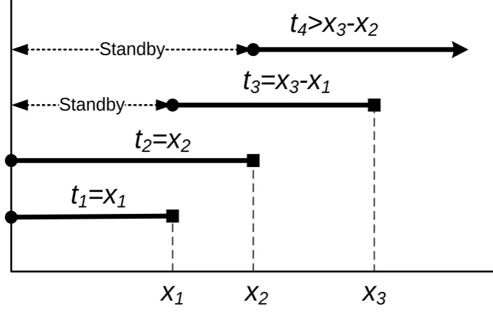
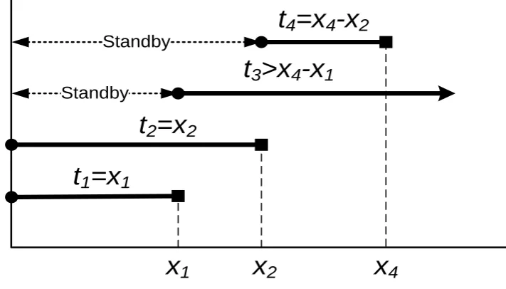
To demonstrate the complexity of system reliability evaluation using a direct method based on sequence of failure events, we consider a 2-out-of-4 cold standby system with perfect switches. The system has a total of 4 components, and it will be in operation as long as there are two good components. In other words, the system reaches a failed state at the event of third component failure. Initially, components 1 and 2 are in operation, and components 3 and 4 are in cold standby. Upon the first component failure due to the failure of either of the working components (component 1 or component 2), component 3 will be kept in operation. Upon the failure of the next component, component 4 will be kept in operation. Therefore, the system reaches a failed state due to one of the following disjoint sequences of failures:

Where xi is the failure time of component i. It is equivalent to the sum of both operational

(59)

The first disadvantage of this method is that when k > 2, the number of sequences with distinct probabilities increases exponentially with (n-k+1) value even when the components are identical. For the 2-out-of-4 system, when the components are identical, the probabilities of sequences (1), (2), (3), and (4) are equivalent to the probabilities of sequences (5), (6), (7), and (8) respectively. However, we still need to find the probabilities for four distinct sequences: (1), (2), (3), and (4). In general, the number of such distinct sequences increases exponentially. For the k-out-of-n system with identical components, the number of distinct sequences is equal to where and

. Therefore, the computational time for evaluating system reliability increases exponentially with the system size.

The second disadvantage of this method is that the probability calculation of each of these sequences involves multiple integrals that are difficult to solve. The third disadvantage of this method is that, for each sequence, the failure times of components must be tracked down to find valid ranges for the integration limits. These are explained further by developing the equations for each of the failure sequences.

Let ti be the operational time of component i at the time of its failure. Note that ti is

different from xi. For example, if component i is kept in the operation at time 100 hours (after

the beginning of the mission) and it fails at time 250 hours, then ti = 150 hours and xi = 250

hours. For sequence (1), we have: t1 = x1, t2 = x2, and t3 = x3-x1. The last event in this

sequence occurs at x3. Hence, the sequence can occur within the mission time t, when x3 < t.

(60)

Standby

x

1

x

2

x

3

t

1

=x

1

t

2

=x

2

t

3

=x

3

-x

1

t

4

>x

3

-x

2

Figure 3.1 – Graphical Representation of Sequence (1)

Let be the probability of sequence i occurring within the mission time. To calculate this probability, for each sequence, we should determine the valid ranges for the operational times of the components. For sequence (1), we have: x1 < x2 < x3. Therefore, valid ranges for

the operational times associated with this sequence are:



Hence, the probability of this sequence occurring within the mission time is:

1 2 3 4 2 3 1 4 4 1 1 2 3 3 1 2 2 0 1 1

1(t) f (t ) f (t ) f (t ) f (t )dt dtdt dt

Q t t t t t t t t t t



      (3.12)

where is the pdf of failure time of component i. This equation can be simplified as:

1 2 3 2 3 1 4 1 1 2 3 3 1 2 2 0 1 1

1(t) f (t ) f (t ) f (t )R (t t t )dt dt dt

Q t t t t t t t   

_



_

 _(3.13)

New Methods for Reliability Evaluation and Enhancement of Power Systems