Article
1
Numerical model for predicting bead geometry and
2
microstructure in Laser Beam Welding of Inconel 718
3
sheets
4
Iñigo Hernando 1, *, Jon Iñaki Arrizubieta 1, Aitzol Lamikiz 1 and Eneko Ukar 1
5
1 University of the Basque Country (UPV/EHU), Dpt. Of Mechanical Engineering - EIB Bilbao, Plaza Torres
6
Quevedo 1, Bilbao, 48013, Spain.
7
* Correspondence: [email protected]; Tel.: +34-946-017-347
8
9
Abstract: A numerical model was developed for predicting the bead geometry and microstructure
10
in Laser Beam Welding of 2 mm thickness Inconel 718 sheets. The experiments were carried out
11
with a 1 kW maximum power fiber laser coupled with a galvanometric scanner. Wobble strategy
12
was employed for sweeping 1 mm wide circular areas for creating the weld seams and a specific
13
tooling was manufactured for supplying protective Argon gas during the welding process. The
14
numerical model takes into account both the laser beam absorption and the melt-pool fluid
15
movement along the bead section, resulting in a weld geometry that depends on the process input
16
parameters, such as feed rate and laser power. The microstructure of the beads was also estimated
17
based on the cooling rate of the material. Features as bead upper and bottom final shapes, weld
18
penetration and dendritic arm spacing were numerically and experimentally analyzed and
19
discussed. The results given by the numerical analysis agree with the tests, making the model a
20
robust predictive tool.
21
Keywords: laser; welding; LBW; model; microstructure; bead seam; wobble strategy; Inconel 718.
22
23
1. Introduction
24
The Laser Beam Welding (LBW) is a material joining technique that apply a laser radiation to
25
melt the base material and create the welding joint. LBW process is related to other traditional
26
welding methods such as Electron Beam Welding (EBW), Tungsten Plasma Arc Welding (PAW) or
27
Inert Gas Tungsten Arc Welding (TIG). LBW apply a high power industrial laser to create a narrow
28
and deep melt pool between the parts to be welded. Laser is a highly concentrated heat source that
29
can be easily automated and installed on industrial welding cells, providing high welding speeds for
30
many industrial applications. Nevertheless, factors such as the laser beam quality or the processed
31
materials have a great influence on the resulting geometry, microstructure and residual stress
32
distribution. Therefore, final results are directly dependent on the process input parameters [1], what
33
means that process parameters must be carefully selected for achieving the desired quality [2].
34
LBW modeling represents a basic tool for predicting the temperature field and giving accurate
35
information about shape of the melt pool and final shape of the bead depending on the process
36
parameters (welding speed, laser power, workpiece geometry, etc.). This fact has a direct impact on
37
reducing the costs derived from experimental tests [3].
38
Modern aircraft engines require materials capable of withstanding high temperatures without
39
lowering their mechanical properties. In order to fulfil this task, nickel-based alloys comprise about
40
50% of the total weight of the engines used in aerospace industry, providing high temperature
41
strength and good resistance against wear or corrosion thanks to their chemical stability [4].
42
Aeronautical structures design and fabrication search for minimum weight models that may put up
43
with several flight work conditions. Since Ni alloys machinability is relatively low and the cost of the
44
material is high, welding techniques present high advantages over machining. On the one hand,
45
welding can be used for building complex structures from smaller parts and, on the other hand,
46
wasted material and chip formation is drastically reduced.
47
Inconel 718 superalloy is widely used in gas turbine components as Tail Bearing Housings
48
(TBH), which have to deal with high temperature gradients and corrosive environments. The strength
49
of the material comes mainly from small ϒ’ and ϒ’’ precipitates that are high in Ni content [5]. On the
50
other hand, despite the Inconel 718 alloy has a reasonably good resistance against weld solidification
51
cracking, it is slightly prone to the appearance of microfissures in the HAZ [6], so LBW is an
52
appropriate joining method as it affects just a narrow zone.
53
Regarding this fact, modeling and study is needed in order to check weld integrity, as LBW is
54
an innovative assembling method both for dispensing rivets and for its good qualities compared to
55
other conventional welding techniques [7]. Besides, LBW has arisen as an alternative to Electron
56
Beam Welding (EBW), which can only be used in a vacuum chamber and requires a more complex
57
fixturing, what results in a much more expensive process.
58
In terms of pores formation, nickel-based alloys with chromium (as Inconel 718) are susceptible
59
to this phenomenon during the welding process, having to resort to protective gases in order to avoid
60
pores [8].
61
The laser power level that material absorbs can be reasonably predicted, so the effects of the heat
62
input may be accurately estimated by a numerical model [9]. The absorptivity of the material
63
represents the ratio of the energy that the workpiece absorbs, it is one of the basis for any heat transfer
64
calculation [10] and hence, modeling must consider this characteristic for any reliable result.
65
Moreover, other effects need to be considered in laser welding processes such as convective and
66
thermocapillary forces that cause deformations during the solidification after the melting phase.
67
These forces are generated due to a decrease of the surface tension of the molten material as
68
temperature increases, which leads to material flow between hot and cold regions [11]. This
69
phenomenon, named as Marangoni effect, has a direct impact on the weld bead geometry [12].
70
Therefore, the model must consider this effect in order to achieve the desired accuracy and predict
71
the welding profile.
72
At the beginning of the LBW technology, Swift-Hook and Gick stated that lasers opened a wide
73
range of possibilities according to deep welds [13] and Klemens declared the many factors as heat,
74
vapor flow, gravity or surface tension are directly connected with the final shape of the seam.
75
Moreover, the need of experimental tests for validating the theoretical heat models took force for
76
identifying unknown factors [14].
77
In the 80s, Mazumder praised the importance of better understanding of the melt pool
78
generation and fluid flow in order to improve the potential of the mathematical models, making them
79
predictive powerful tools [10]. In the same way, Goldak et al. asserted that the prediction of aspects
80
such as the strength of the welded structures, which is directly related to residual stress or distortions,
81
called for precise analysis of the thermal cycles for further modeling [15].
82
Afterwards, Bonollo et al. assured that the laser welding dynamics were not entirely understood,
83
despite theoretical evaluation and subsequent experimental validation had enabled to develop the
84
comprehension of the LBW technique [16]. This statement was confirmed by Kaplan et al., who
85
placed value on modeling for improving the physical understanding of the LBW process [17].
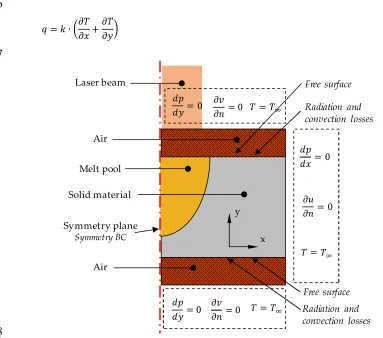
86
Ducharme et al., for their part, stood out that modeling allowed to demonstrate the relation between
87
the keyhole and the melt pool [18].
88
Sudnik et al. alleged the need of new theoretical work in order to better the laser welding process
89
as well as its control and defects description. This was grounded on the fact that many heat
90
conduction models did not achieve the desired accuracy when predicting the weld bead geometry
91
[19]. Nevertheless, Tsirkas et al. pointed the difficulty of modeling the welding process, as thermal,
92
mechanical and metallurgical phenomena take place at the same time [20]. Furthermore, Gery et al.
93
concluded that the experimental work is mandatory for determining relations between heat source
94
models and subsequent empirical testing [21].
95
Later, Kazemi and Goldak continued maintaining the idea that modeling the laser keyhole
96
temperature fields [3]. In turn, Zhao et al. affirmed that the coexistence of three different phases
98
(plasma, liquid and solid) added to the complex keyhole behavior and the forces acting in the weld
99
pool made modeling still difficult [22].
100
Likewise, Kubiak et al. underlined the necessity of an innovative focusing on the theory and
101
numerical solution techniques used for the LBW, as this process offers characteristic heat
102
distributions compared to traditional welding methods [23]. However, Zhang et al. pointed that
103
despite of the advances in laser deep penetration knowledge due to numerical simulation, yet many
104
issues remain unexplored [24].
105
For this reason, it is concluded that there is a need in the aerospace industry to develop a model
106
that predicts the geometry of the resulting joint when welding thin Inconel 718 plates. Therefore, a
107
model that considers the melt pool dynamics during the welding process is developed. In addition,
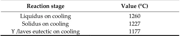
108
the obtained results have been experimentally validated under different conditions. Moreover, the
109
numeric tool is capable of predicting the generated microstructure based on the thermal field
110
variations during the process.
111
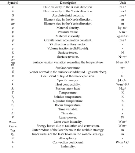
Table 1. Employed symbols and nomenclature.
112
Symbol Description Unit
u Fluid velocity in the X axis direction. m·s-1
v Fluid velocity in the Y axis direction. m·s-1
U Absolute fluid velocity. m·s-1
∆ Element size in the X axis direction. m
∆ Element size in the Y axis direction. m
Material density. kg· m-3
Pressure value. N·m-2
Material viscosity. kg·m-1·s-1
Gravitational acceleration constant. m·s-2
⃑ Y+ direction unitary vector. -
Volume fraction (solid/liquid). -
Surface forces. N
Surface tension. N· m-1
Surface tension variation regarding the temperature. N· m-1·K-1
Surface curvature. m-1
⃗ Vector normal to the surface (solid/liquid – gas interface). - Coefficient of liquid thermal expansion. K-1
Specific energy. J·kg-1·c
Heat conductivity. W·m-1⋅K-1
Fusion latent heat. J·kg-1
Temperature. K
Solidus temperature. K
Liquidus temperature. K
∞ Room temperature. K
t Time variable. s
Δt Time step. s
Laser power. W
Laser beam intensity. W·m-2
Energy losses due to radiation and convection. W·m-2
Outer radius of the laser beam in the wobble strategy. m Inner radius of the laser beam in the wobble strategy. m
Absorptivity. -
ℎ Convection coefficient. W· m-2 K-1
Stefan-Boltzmann coefficient. W· m-2 K-4
Angle between the laser beam and the normal vector to the
surface rad
Welding feed rate. mm·s-1
Peripheral speed in the wobble operation mm·s-1
113
2. Developed model
114
2.1 Model Basis
115
The proposed model is based on solving the continuity (1), momentum (2) and energy
116
conservation (3) equations in order to obtain the pressure, velocity and temperature fields of each
117
element respectively. The coupled pressure-velocity equations are solved using the SIMPLE
118
algorithm proposed by Patankar [25] and a fully implicit scheme is used.
119
120
+ ( ∙ ) + ( ∙ ) = 0 (1)
( ∙ ф) + ( ∙ ∙ ф) + ( ∙ ∙ ф) = − + ∙ ф − + ∙ ф + (2)
( ∙ ∙ ) + ( ∙ ∙ ∙ ) + ( ∙ ∙ ∙ ) = ∙ + ∙ + (3)
121
The momentum generation term (Sm) includes the buoyancy force (Sb) generated as a
122
consequence of the density difference and the velocity reduction term (Sd) introduced in those
123
elements where the material is in solid state. Material is considered completely rigid and
124
incompressible when it is in solid state, therefore, the velocity of the material in the solid region is
125
zero. This is modeled by the second term in equation (4), where the parameter has a zero value in
126
the solid and a unit value in the liquid. In order to avoid zeros in the denominator, C=106 and e0=10-3
127
values are adopted [25].
128
129
= + = ∙ ∙ ∙ ( − ). ⃑ − ∙ (1 − )
+ ∙ (4)
130
Regarding the energy generation term (Se), equation (5), includes the latent heat (SL) and the heat
131
exchange at the substrate surface (SC). Inside this second term, the energy radiated by the laser beam
132
(qlaser) and the heat losses due to radiation and convection (qlosses) are included. As no material
133
vaporization is expected, the model includes only the fusion latent heat, which is defined in equation
134
(6).
135
136
= + = + − (5)
= ∙ = ∙ ∙ (6)
137
The energy input at the surface can be approximated as a ring-type source, generated by a
fast-138
moving laser spot that follows a wobble strategy, as it is shown in Figure 1. Therefore, the energy
139
input in a surface element located at an x and y planar distance from the laser beam center point is
140
defined by means of equation (7). As the free surface can deform freely, the absorptivity value ( ) is
141
free surface ( ). On the other hand, radiation and convection losses at the surface of the substrate are
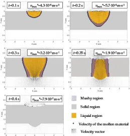
143
described by equation (8), where n is the number of free-faces of a certain element located on the
144
surface.
145
146
=2 ∙ · ( ) ∙
∙ ( − ) (7)
= · [ℎ ∙ ( − ) + ∙ ∙ ( − )] (8)
147
148
149
Figure 1. Instantaneous laser spot and modeled laser beam in wobble strategy
150
151
The model considers conduction and diffusion as heat transfer mechanisms within the material.
152
Moreover, the Volume of Fluid (VOF) equation (9) is solved to determine the material movement and
153
the variation of the free surface. For tracking the interface, the interface capturing method is used
154
because, unlike other methods, does not introduce restrictions to the evolution of the free surface.
155
This method gives the position of the boundary between the different phases by using a scalar
156
transport variable. The volume fraction ( ) becomes a zero value in the gas and a unit value in the
157
base material (solid or liquid). So, the interface is defined as the transition zone where takes a value
158
between zero and the unit.
159
160
+ ( ∙ ) = 0 (9)
161
The residue value to ensure the convergence of the results is set to a 10-3 value between two
162
subsequent iterations [25]. The same criteria is used for mass, momentum, energy conservation and
163
VOF equations.
164
2.2 Initial and boundary conditions
165
In order to start the simulation, the initial temperature of all elements must be defined. since no
166
preheating stage has been considered, all nodes are supposed to be at room temperature ( =298 K).
167
Therefore, the whole substrate is in solid state at the initial stage and all the elements have a
168
zero-velocity value.
169
Velocity, pressure and temperature values are determined at the limits of the model by means
170
of the boundary conditions, see Figure 2. On the one hand, a zero-pressure gradient condition is
171
stablished in all the boundaries. On the other hand, a zero-velocity vector variation condition is
172
stablished in all boundary faces. Lastly, in terms of temperature boundaries, the nodes next to the
173
control volume are forced to be at room temperature ( =298 K). This is equivalent to consider a first
174
specie or Dirichlet boundary condition, equation (10).
175
vp
s
rout rin
vf Instantaneous
laser spot
Modeled laser beam
Z
176
= ∙ + (10)
177
178
Figure 2. Applied boundary conditions for modeling the welding process.
179
180
With the aim of reducing unnecessary computational cost and based on the symmetric nature of
181
the modeled problem, just half of the volume is simulated. The following boundary conditions are
182
set in the symmetry plane:
183
184
= 0 ; = 0 ; = 0 (11)
2.3 Surface forces
185
Movement of the molten material is generated due to surface forces, see equation (12). On the
186
one hand, a force normal to the surface takes place due to the curvature developed by the interface
187
between the air and substrate. On the other hand, Marangoni forces are generated because of the
188
surface stress variation regarding the temperature variation. Besides, buoyancy forces are included
189
in the model, which generate a downwards force. All forces considered in the model are shown in
190
Figure 3.
191
192
= ∙ ∙ ⃗ + [ − ⃗ ∙ ( ⃗ ∙ )] (12)
Melt pool
Solid material
Symmetry plane Symmetry BC
Radiation and convection losses
= 0 =
Free surface
Air Laser beam
= 0 =
= 0
= 0
=
= 0 = 0
x y
Air
Radiation and convection losses
193
Figure 3. Material movement due to the surface and buoyancy forces.
194
195
2.4 Microstructure
196
The internal structure of material after melting and solidifying depends directly on the process
197
cooling rate. When the temperature drops below the liquidus temperature (TL), columnar dendritic
198
microstructure is formed until the solidus temperature (TS) is reached. This temperature
phase-199
change range is named as the mushy zone [26].
200
The interplanar spacing between different dendrites can be estimated based on the cooling rate
201
and the boundary temperatures where the material undergoes the phase changes, which are the TL
202
and the ϒ/laves eutectic temperature (Te). At this juncture, dendritic columns grow mainly in the
203
energetically favorable crystallographic directions, forming the principal axis and, to a lesser extent,
204
in the other transverse secondary directions [6]. The secondary dendrite arm spacing (SDAS) is
205
measured in this research tests for subsequent thermal model validation by means of equation (13).
206
To this end, the mean values are calculated based on ten different measurements for each analyzed
207
welding bead. SDAS is measured in m and C is a constant that depends on the material. For the
208
specific case of the Inconel 718 this constant takes a value of 10 [27].
209
210
= · − (13)
211
The Inconel 718 is a widely used and studied material and therefore, many authors have
212
contributed with their research to the determination of these reaction temperatures. In the present
213
investigation, the values given by Eiselstein for the cooling case are considered [28]: 1260 °C and
214
1177 °C for the liquidus temperature (TL) and the ϒ/laves eutectic temperature (Te), respectively.
215
Table 2. Inconel 718 cooling temperatures.
216
Reaction stage Value (°C)
Liquidus on cooling 1260
Solidus on cooling 1227
ϒ /laves eutectic on cooling 1177
217
3. Proposed methodology for the model validation
218
Validation has been carried out using FL010 1kW fiber laser from Rofin FL010 with an ouput
219
fiber of 100 µm coupled to galvanometric scan head hurrySCAN® 25 from SCANLAB with a
220
maximum workspace of 120 x 120 mm and maximum feed rate of 10,000 mm·s-1. Scan head allows
221
fast movements of the laser beam because of the low inertia of the moving mirrors, giving as result
222
high velocities and accelerations without losing positioning accuracy. Therefore, the laser beam
223
motion is fast enough to consider as a ring-type spot of 1 mm diameter that moves at a feed rate
224
MARANGONI FORCES BUOYANCY FORCES CURVATURE FORCES
speed. In this case, a wobble strategy is used for the welding process, see Figure 4. This method allows
225
to fill an area by describing rings, so a suitable relation between the feed rate ( ) and the peripheral
226
speed ( ) is implemented for achieving minimum overlap and no space among consecutive rings.
227
So, the laser spot must spend the same time for tracing a loop (orbital motion) and for advancing a
228
spot diameter distance (linear movement).
229
230
Figure 4. Wobble scanning technique employed for the welding operation
231
232
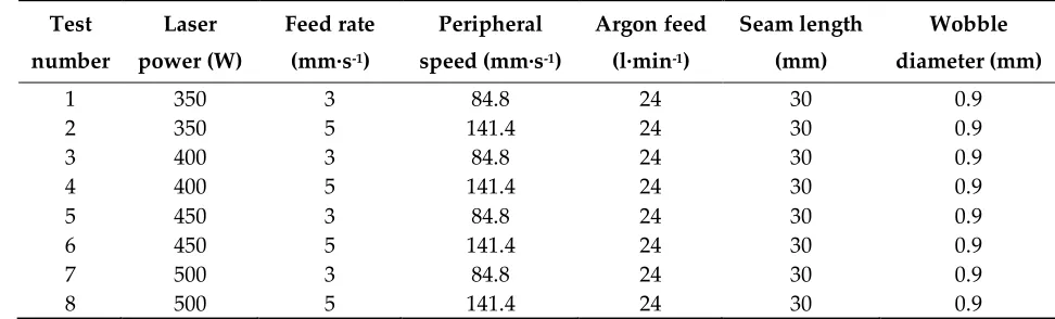
The selected continuous laser powers for welding the 2 mm thickness Inconel 718 sheets are
233
350 W, 400 W, 450 W and 500 W in combination with two different feed rates: 3 mm·s-1 and 5 mm·s-1.
234
The seam length is of 30 mm, enough to ensure steady state is achieved during welding track.
235
Afterwards, all the samples are cut at a 20 mm distance from the beginning of the weld, encapsulated
236
and polished for Marble solution etching, Figure 5. The geometry of the weld beads is revealed by
237
this chemical attack in order to analyze their cross shape and compare them with the results provided
238
by the model. Moreover, secondary dendrite arms spacing (SDAS) in the samples is measured for the
239
cases where the minimum and maximum powers are applied (350 W and 500 W, respectively).
240
Finally, the measured SDAS is compared with the values predicted by the numerical model.
241
242
243
244
Figure 5. Upper view (left), cross section (center) and detail of the microstructure (right) of the Test 6.
245
Table 3. Process parameters for the different tests
246
Test
number
Laser
power (W)
Feed rate
(mm·s-1)
Peripheral
speed (mm·s-1)
Argon feed
(l·min-1)
Seam length
(mm)
Wobble
diameter (mm)
1 350 3 84.8 24 30 0.9
2 350 5 141.4 24 30 0.9
3 400 3 84.8 24 30 0.9
4 400 5 141.4 24 30 0.9
5 450 3 84.8 24 30 0.9
6 450 5 141.4 24 30 0.9
7 500 3 84.8 24 30 0.9
8 500 5 141.4 24 30 0.9
Instantaneous laser spot
Modeled laser beam
Z
X Y
vp
1
m
m
3.1. Model parameters
247
The modeled cross section has an 8x4 mm size in the X and Y directions, respectively. Notice
248
that in x=0 a symmetry boundary condition is considered (see Figure 2). The distant face in this
249
direction must be placed at a far enough from the laser beam source in order to avoid any
250
disturbances in the generated thermal field, but without putting far away in order to avoid,
251
computational cost increased in vain. On the other hand, in the Y direction, a 1 mm layer of air is
252
considered below and above the sheets to be welded, which is enough for allowing the free
253
movement of the air-filled elements.
254
Defining an appropriate element size is critical when achieving a good relation between
255
accuracy and computational cost. After testing with 0.1, 0.075, 0.05, 0.025 mm size elements and
256
evaluating the obtained accuracy and the elapsed time required for the simulation, it is considered
257
that a 0.05 mm element size is the optimum value. As it can be observed in Figure 6, after simulating
258
the Test 4 with different element sizes, an error below 5% is obtained with a 0.05mm element size
259
when the depth of the weld bead is measured, together with an elapsed time of 392.95 s.
260
261
262
Figure 6. Variation of the elapsed time required for running the simulation and the obtained error
263
compared with the experimentally measured depth of the weld bead as the element size varies for the case of
264
the Test 4.
265
266
Besides, obtained results depend on the time increment used in simulation. For the present
267
validation, a 0.001s time step is used. A higher time step means that fewer steps are required for
268
sweeping the desired time interval, whereas a smaller time step means the opposite. However, higher
269
time step results in higher variations of the pressure and velocity fields, and consequently, the
270
number of required iterations before achieving the desired accuracy is also increased. In addition,
271
instabilities may appear, resulting in the necessity of lowering the under-relaxation factors used in
272
the SIMPLE algorithm (0.8 and 0.5 for the pressure and velocities calculation, respectively).
273
The cooling stage has direct impact in the final shape of the melt pool [29], as well as the
274
developed microstructure [30]. Therefore, an extra time is simulated after the laser passes over the
275
modeled cross section is in order to analyze the cooling stage and the solidification of the material. A
276
total simulation times of 1.0 s and 0.6 s are defined for the tests where 3 mm·s-1 and 5 mm·s-1 feed rates
277
are used, respectively.
278
3.2. Materials
279
Inconel 718 sheets with a 2 mm thickness are used for LBW tests. This value is similar to the
280
thickness of the sheets used in the aerospace gas turbines.
281
282
283
284
0 5 10 15 20 25 30
0 500 1000 1500 2000 2500 3000 3500 4000 4500
E
rr
o
r
[%
]
Element size [mm]
0.025 0.05 0.075 0.1
Elapsed time [s] Error [%]
E
la
p
se
d
ti
m
e
[s
Table 4. Inconel 718 composition (% w.t.) ([31])
285
Al B C Co Cr Cu Fe Mn Mo Ni
0.55 0.004 0.054 0.28 18.60 0.05 18.60 0.24 3.03 52.40
P S Si Ti Nb Ta Bi Pb Ag
<0.005 <0.002 0.06 0.98 4.89 <0.05 <0.00003 <0.0005 <0.0002
286
Table 5. Properties of Inconel 718 (Average thermo-physical properties of Inconel 718 [32])
287
Definition Unit Value
Melting range (Tm) K 1533–1609
Density (ρ) Kg·m-3 8190
Specific heat (c) J·kg-1·K-1 435
Conductivity (k) W·m-1·K-1 8.9
Latent heat fusion (SL) J·kg-1 210x103
Density ( ) (liquid phase) Kg·m-3 7400
Specific heat ( ) (liquid phase) J·kg-1·K-1 720
Conductivity (kL) (liquid phase) W·m-1·K-1 29.6
288
The developed model is two-dimensional, since most of the laser welding tracks can be
289
considered as longitudinal tracks with constant section. Authors like Casalino concluded in their
290
research the suitability of using a two-dimensional model for simulating the LBW process [2].
291
However, the heat transfer in the experimental situation is tridimensional (including lateral and
292
longitudinal conduction). Therefore, a tridimensional heat transfer is considered in the model. Thus,
293
heat transfer due to conductivity and convection is taken into account in the X, Y and in Z directions,
294
assuming the symmetry in the X direction.
295
296
3.3. Experimental setup
297
Test parts are clamped to avoid distortions caused by thermal expansion or contraction during
298
the melting and solidification process, Figure 7, which could cause misalignment in the weld zone.
299
300
301
Figure 7. Test parts placing examples: Properly clamped (a) and simply supported (b)
302
303
The welding process is performed with an argon 2X protective atmosphere (99.995% of argon
304
purity). The argon gas is inserted through four slots situated in four cylindrical tubes, two pointing
305
to the welding upper surface and the two others to the bottom one, which ensures a homogenous
306
supply all along the seam path (see Figure 8). The argon supply is of 24 l·min-1 (6 l·min-1 through each
307
80 mm x 2 mm rectangular slot).
308
309
310
Figure 8. a) Experimental setup for ensuring the protective atmosphere during the LBW tests;
311
b) Frontal and lateral schematic views.
312
4. Results
313
The developed model calculates the temperature field at different time steps as the laser beam
314
passes over the modeled section. As a consequence of the temperature gradients generated within
315
the molten material, Marangoni forces are generated and lead to creation of convection currents, see
316
Figure 9. The size of the melt pool is increased as the interaction time increases and can reach a
317
situation in which the whole thickness of the Inconel 718 sheet is melted (this situation occurs at a
318
t=0.28 s instant in Test 5, 450 W laser power and vf=3 mm·s-1) and molten material starts to drop due
319
to gravity forces. After the laser beam passes by the modeled cross section and there is no external
320
heat input, the material solidifies, resulting in the final shape of the generated weld bead. This final
321
shape together with the area melted during the whole process is compared with the experimental
322
324
Figure 9. Evolution of the welding section and material velocity in Test 5 as the laser beam passes.
325
4.1. Analysis of the geomettry of the weld beads
326
In order to validate the developed model, the weld beads from the different tests are measured
327
taking into account the following features (see Figure 10): penetration depth (named with the letter
328
D), weld bead width (named with the letter W) and height both in the crown and the root (named
329
with the letters A and R, respectively). Due to the movement of the molten material during the
330
welding process, the surface tension generates fillets or groovy shapes at the weld crown. The molten
331
material also may stick out at the root when the penetration is complete, forming sagged geometries
332
beyond the lower surface. The established sign criterion is positive (+) for fillets and saggings and
333
negative (-) for grooves.
334
335
Figure 10. Scheme of the different cross sections of the weld bead.
336
337
Table 6. Geometrical validation of the model (width and depth).
338
Test number
Crown Width (W) Depth (D)
Experimental (mm)
Model (mm)
Error (%)
Experimental (mm)
Model (mm)
Error (%)
1 2.16 2.30 6.38 2.00 2.00 0.00
2 1.98 1.80 9.09 1.09 1.05 3.93
3 2.42 2.50 3.52 2.00 2.00 0.00
4 2.07 2.00 3.19 1.30 1.33 2.47
5 2.56 2.60 1.76 2.00 2.00 0.00
6 2.40 2.20 8.37 1.72 1.75 1.74
7 2.82 2.62 7.13 2.00 2.00 0.00
8 2.61 2.35 9.82 2.00 2.00 0.00
FILLET
GROOVE
CROWN CROWN
SAG
ROOT R (+)
W
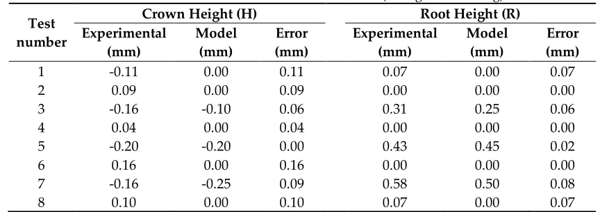
Table 7. Geometrical validation of the model (fillet-groove and sag)
339
Test number
Crown Height (H) Root Height (R)
Experimental (mm)
Model (mm)
Error (mm)
Experimental (mm)
Model (mm)
Error (mm)
1 -0.11 0.00 0.11 0.07 0.00 0.07
2 0.09 0.00 0.09 0.00 0.00 0.00
3 -0.16 -0.10 0.06 0.31 0.25 0.06
4 0.04 0.00 0.04 0.00 0.00 0.00
5 -0.20 -0.20 0.00 0.43 0.45 0.02
6 0.16 0.00 0.16 0.00 0.00 0.00
7 -0.16 -0.25 0.09 0.58 0.50 0.08
8 0.10 0.00 0.10 0.07 0.00 0.07
340
The numeric model shows an error below 4% regarding to the weld bead penetration depth and
341
a less than 10% error for the crown width, Table 6. For both the crown and root height prediction, the
342
model shows an error smaller than 0.2 mm, Table 7. In Figure 11 a comparison between the modeled
343
and the measured cross sections is shown for the Tests 1-8.
344
345
4.2. Microstructure validation
347
The microstructure is studied for the Tests 1, 2, 7 and 8 and in each case, as detailed in Figure 12,
348
two different areas are studied for validating the model prediction of the SDAS value. The first one
349
(M1) is located near the boundary between the weld bead and the HAZ and it is the first area where
350
the material solidifies after its melting, whereas the second one (M2) is placed in the center of the
351
bead.
352
353
Figure 12. Secondary dendrite arm spacing (SDAS) of Test 8 together with the experimental
354
microstructure details in regions M1 and M2.
355
The analysis of the experimental tests is carried out by a Leica DCM 3D microscopy with 100X
356
magnification. For each study zone, the SDAS measurements are performed and the average value is
357
calculated, which is compared with the results given by the numerical model, see Table 8. The
358
maximum error between the predicted SDAS values and the measured ones is below 1.5 microns,
359
which means that there is a good agreement between the model and the experimental process. Also,
360
since the microstructure depends on the cooling rate, which depends on the variation of the thermal
361
field, so, it can be concluded that the model predicts the temperature field accurately during the LBW
362
process.
363
Table 8. Microstructure validation of the model.
364
Test number
Area M1 Area M2
Model (m)
Experimental (m)
Error (m)
Model (m)
Experimental (m)
Error (m)
1 2.71 3.19 -0.48 2.77 3.70 -0.93
2 2.21 3.05 -0.84 2.04 2.58 -0.54
7 2.31 3.78 -1.47 2.82 4.25 -1.43
8 2.08 3.54 -1.46 1.83 2.63 -0.80
5. Conclusions
365
In the present work, a numerical model for predicting the weld bead in the LBW process is
366
developed and validated under different process parameters. According to the obtained results, the
367
following conclusions can be drawn:
368
(1) The developed model represents accurately the weld beads generated under different process
369
parameters. In all cases, the maximum error is lower than the 10% regarding the weld bead
370
width and depth, which ensures a high agreement between the model and the tests.
371
(2) The developed tool is valid for modeling not only the melt pool dynamics, but also the drop of
372
the molten material once the laser beam melts the whole thickness of the Inconel 718 sheets.
373
An error below 0.2 mm is detected between the model and the experimental results in the
374
crown and root heights of the weld bead. However, the model resulted incapable of predicting
375
(3) After comparing the microstructure measured in the experimental tests and the values given
377
by the model, it is concluded that the model gives the SDAS with an error below 1.5 microns.
378
The two different areas that are analyzed (M1 and M2) show that the SDAS in the test tubes is
379
slightly higher than the value given by the model. Hence, it is concluded that the predicted
380
cooling rate is also somewhat higher than the real one. This can be originated by the symmetry
381
assumption or the two-dimensional solving of the melt pool dynamics, whereas the physical
382
problem is three-dimensional.
383
Therefore, the proposed model results to be appropriate for modeling the LBW process and can
384
be used as a predictive tool for simulating weld beads before carrying out real tests. Therefore, it has
385
a direct application on aerospace industry and specifically in Inconel 718 welds.
386
Author Contributions: Iñigo Hernando conceived, designed and performed the experiments; Iñigo Hernando
387
and Jon Iñaki Arrizubieta developed the numerical model; Eneko Ukar and Aitzol Lamikiz analyzed the data.
388
Aitzol Lamikiz reviewed previous works related with the subject. Iñigo Hernando and Jon Iñaki Arrizubieta
389
wrote the paper.
390
Funding: This research received no external funding.
391
Acknowledgments: Thanks are addressed to H2020-FoF13-2016 PARADDISE project (contract number 723440).
392
Special thanks are addressed to the University of the Basque Country (UPV-EHU) for the funding support
393
received from the contracting call for the training of research staff in UPV-EHU 2015.
394
Conflicts of Interest: The authors declare no conflict of interest.
395
References
396
1. Liu, S.; Mi, G.; Yan, F.; Wang, C.; Jiang, P.; Correlation of high power laser welding parameters with real
397
weld geometry and microstructure. Optics & Laser Technology, 2017, 94, 59-67.
398
DOI:10.1016/j.optlastec.2017.03.004
399
2. D’Ostuni, S.; Leo, P.; Casalino, G. FEM Simulation of Dissimilar Aluminum Titanium Fiber Laser Welding
400
Using 2D and 3D Gaussian Heat Sources. Metals, 2017, 7, 307. DOI:10.3390/met7080307
401
3. Kazemi, K.; Goldak, J.A. Numerical simulation of laser full penetration welding. Computational Materials
402
Science, 2009, 44, 841-849. DOI:10.1016/j.commatsci.2008.01.002
403
4. Venkatesan, K.; Ramanujam, R.; Kuppan, P. Parametric modeling and optimization of laser scanning
404
parameters during laser assisted machining of Inconel 718. Optics & Laser Technology, 2016, 78, 10-18.
405
DOI:10.1016/j.optlastec.2015.09.021
406
5. Anderson, M.; Patwa, R.; Shin, Y.C. Laser-assisted machining of Inconel 718 with an economic
407
analysis. International Journal of Machine Tools and Manufacture, 2006, 46, 1879-1891.
408
DOI:10.1016/j.ijmachtools.2005.11.005
409
6. Ram, G.D.J.; Reddy, A.V.; Rao, K.P.; Reddy, G.M.; Sundar, J.K.S. Microstructure and tensile properties of
410
Inconel 718 pulsed Nd-YAG laser welds. Journal of Materials Processing Technology, 2005, 167, 73-82.
411
DOI:10.1016/j.jmatprotec.2004.09.081
412
7. Steen, W.M.; Mazumder, J. Laser material processing, 4th ed.; Springer: London, England, 2010. ISBN
978-1-413
84996-061-8
414
8. Davis, J.R. ASM specialty handbook: nickel, cobalt, and their alloys. ASM International: Ohio, USA, 2000.
415
9. Dowden, J.M. The mathematics of thermal modeling: an introduction to the theory of laser material
416
processing, Chapman & Hall/CRC: Boca Raton, USA, 2001. ISBN 978-1-58488-230-5
417
10. Mazumder, J. Laser welding. In Laser materials processing, 1st ed.; Bass, M.; Elsevier: New York, USA, 1983;
418
Volume 3, pp. 120-200. ISBN 0-444-86396-6
419
11. Brown, M.S; Arnold, C.B. Fundamentals of Laser-Material Interaction and Application to Multiscale
420
Surface Modification. In Laser precision microfabrication, 1st ed.; Sugioka, K.; Meunier, M.; Piqué,
421
A.; Springer: London, England. 2010. ISBN 978-3-642-10522-7
422
12. Mills, K. C., Keene, B.J.; Brooks, R.F.; Shirali, A. Marangoni effects in welding. Philosophical Transactions of
423
the Royal Society a Mathematical Physical and Engineering Sciences, 1998, 356, 911-926.
424
DOI: 10.1098/rsta.1998.0196
425
14. Klemens, P. G. Heat balance and flow conditions for electron beam and laser welding. Journal of Applied
427
physics, 1976, 47, 2165-2174. DOI:10.1063/1.322866
428
15. Goldak, J.; Chakravarti, A.; Bibby, M. A new finite element model for welding heat sources. Metallurgical
429
transactions B, 1984, 15, no 2, p. 299-305. DOI: 10.1007/BF02667333
430
16. Bonollo, F.; Tiziani, A.; Zambon, A. Model for CO2 laser welding of stainless steel, titanium, and nickel:
431
parametric study. Materials Science and Technology, 1993, 9, 1137-1144. DOI:10.1179/mst.1993.9.12.1137
432
17. Kaplan, A. A model of deep penetration laser welding based on calculation of the keyhole profile. Journal
433
of Physics D: Applied Physics, 1994, 27, 1805-1814. DOI:10.1088/0022-3727/27/9/002
434
18. Ducharme, R.; Williams, K.; Kapadia, P.; Dowden, J.; Steen, B.; Glowacki, M.. The laser welding of thin
435
metal sheets: an integrated keyhole and weld pool model with supporting experiments. Journal of physics
436
D: Applied physics, 1994, 27, 1619-1627. DOI:10.1088/0022-3727/27/8/006
437
19. Sudnik, W.; Radaj, D.; Breitschwerdt, S.; Erofeew, W. Numerical simulation of weld pool geometry in laser
438
beam welding. Journal of Physics D: Applied Physics, 2000, 33, 662-671. DOI:10.1088/0022-3727/33/6/312
439
20. Tsirkas, S.A.; Papanikos, P.; Kermanidis, Th. Numerical simulation of the laser welding process in
butt-440
joint specimens. Journal of materials processing technology, 2003, 134, 59-69.
441
DOI:10.1016/S0924-0136(02)00921-4
442
21. Gery, D.; Long, H.; Maropoulos, P. Effects of welding speed, energy input and heat source distribution on
443
temperature variations in butt joint welding. Journal of materials processing technology, 2005, 167, 393-401.
444
DOI:10.1016/j.jmatprotec.2005.06.018
445
22. Zhao, H.; Niu, W.; Zhang, B.; Lei, Y.; Kodama, M.; Ishide, T. Modelling of keyhole dynamics and porosity
446
formation considering the adaptive keyhole shape and three-phase coupling during deep-penetration laser
447
welding. Journal of Physics D: Applied Physics, 2011, 44, 485302. DOI:10.1088/0022-3727/44/48/485302
448
23. Kubiak, M, Piekarska, W.; Saternus, Z.; Domanski, T. Numerical prediction of fusion zone and heat affected
449
zone in hybrid Yb: YAG laser+ GMAW welding process with experimental verification. Procedia
450
Engineering, 2016, 136, 88-94. DOI: 10.1016/j.proeng.2016.01.179
451
24. Zhang, L.J.; Zhang, J.X.; Gumenyuk, A.; Rethmeier, M.; Na, S.J. Numerical simulation of full penetration
452
laser welding of thick steel plate with high power high brightness laser. Journal of materials processing
453
technology, 2014, 214, 1710-1720. DOI:10.1016/j.jmatprotec.2014.03.016
454
25. Patankar, S.V. Numerical heat transfer and fluid flow, 1st ed.; McGraw-Hill, 1980. ISBN-13:978-0891165224
455
26. Voller, V.R.; Prakash, C. A fixed grid numerical modelling methodology for convection-diffusion mushy
456
region phase-change problems. International Journal of Heat and Mass Transfer, 1987, 30, 1709-1719.
457
DOI:10.1016/0017-9310(87)90317-6
458
27. Patel, A.D.; Murty, Y.V. Effect of cooling rate on microstructural development in alloy 718. International
459
symposium; 5th, Superalloys; Superalloys 718, 625, 706 and various derivatives, Warrendale (USA), 2001,
460
123-132.
461
28. Antonsson, T.; Fredriksson, H. The effect of cooling rate on the solidification of Inconel 718. Metallurgical
462
and Materials Transactions B, 2005, 36, 85-96. DOI:10.1007/s11663-005-0009-0
463
29. Saldi, Z. S.; Kidess, A.; Kenjeres, S.; Zhao, C.; Richardson, I.M., Kleijin, C.R. Effect of enhanced heat and
464
mass transport and flow reversal during cool down on weld pool shapes in laser spot welding of
465
steel. International Journal of Heat and Mass Transfer, 2013, 66, 879-888.
466
DOI:10.1016/j.ijheatmasstransfer.2013.07.085
467
30. Zhang, Y. N.; Cao, X.; Wanjara, P. Microstructure and hardness of fiber laser deposited Inconel 718 using
468
filler wire. The International Journal of Advanced Manufacturing Technology, 2013, 69, 2569-2581.
469
DOI:10.1007/s00170-013-5171-y
470
31. Haynes International. Material Sales order 810002010-0; Customer reference 20PPO009192; Report No.
471
20151117074
472
32. Mills, K.C. Recommended values of thermophysical properties for selected commercial alloys, 1st ed.; Woodhead