Actively Secure Setup for SPDZ
Dragos Rotaru1,2[0000−0002−1767−3725], Nigel P. Smart1,2[0000−0003−3567−3304], Titouan
Tanguy1[0000−0002−7965−620X], Frederik Vercauteren1[0000−0002−7208−9599], and Tim Wood1,2[0000−0003−1082−4321]
1
imec-COSIC, KU Leuven, Leuven, Belgium.
2 University of Bristol, Bristol, UK.
[email protected], [email protected],
[email protected], [email protected], [email protected]
Abstract. We present the first actively secure, practical protocol to generate the distributed secret keys needed in the SPDZ offline protocol. As an added bonus our protocol results in the resulting distribution of the public and secret keys is such that the associated SHE ‘noise’ analysis is the same as if the distributed keys were generated by a trusted setup. We implemented the presented protocol for distributed BGV key generation within theSCALE-MAMBA framework. Our method makes use of a new method for creating doubly (or even more) authenticated bits in different MPC engines, which has applications in other areas of MPC-based secure computation. We were able to generate keys for two parties and a plaintext size of 64 bits in around five minutes, and a little more than eighteen minutes for a 128 bit prime.
Keywords: MPC·Somewhat Homomorphic Encryption·Key Generation
1
Introduction
The SPDZ protocol for Multi-Party Computation (MPC) was introduced in 2012 [12]. This protocol is in the pre-processing family of protocols which are actively secure-with-abort for a dishonest majority of participants. Due to many improvements over the intervening years it provides a highly efficient mechanism to perform MPC for an arbitrary number of participants. However, the protocol comes with a major security issue: namely that it seems to require a trusted setup. This trusted setup is the creation of a public key for the Brakerski-Gentry-Vaikuntanathan [7] (BGV) homomorphic encryption scheme in which the private key is securely distributed amongst the n-parties.
In the original SPDZ paper [12] this was assumed to come from some trusted setup. In the follow up paper [11] a covertly secure protocol for generating a suitably distributed set of private keys, and the associated public key was introduced. However, this came with a number of disadvantages, as well as the reduction to just covert security. In particular the distributions of the underlying public keys were different from those one could attain via a trusted setup, which led to a more complicated noise analysis, and (more importantly) larger parameters which results in less efficient protocols.
The problem of producing distributed key generation for an SHE/FHE scheme arises in other contexts. For example, inspired by Gentry’s FHE based passively secure low round complexity MPC protocol from [15], various authors have looked at distributed decryption for FHE/SHE schemes. Each of these proposals needs a method to perform a distributed key generation phase. In [4] the authors present a key generation method for a distributed SHE scheme using variousΣ-protocols. To our knowledge this has never been implemented, and the methodology produces a key generation which is different from what would be done via a trusted setup. In [25] a passively secure distributed key generation method is used for threshold SHE schemes, again producing a distribution different from that one would have in a purely trusted setup. Our protocol could also be used in these situations to instantiate MPC based on FHE.
In [9] introduce a variant of SPDZ, called SPDZ2k, for the case of MPC over the ring Z2k. The offline phase in this latter work is based on MASCOT. However, in [26] the au-thors present an offline protocol based on distributed FHE for SPDZ2k. Our distributed key generation method will also work for this protocol as well.
Our Contrubution: In this paper we show present the first practicalactively securedistributed key generation method for SPDZ. As an added bonus our method results in virtually identical secret key distributions as in the trusted setup case. In particular the noise analysis for the resulting public key is identical to that one would have if using a trusted setup. Our protocol is also relatively simple, although it does make use of complex generic MPC technology. In particular, our protocol generates a public/private key with exactly the same distribution as the ideal trusted setup does in the SCALE-MAMBA system3, bar the fact we generate secret keys with expected Hamming weight h as opposed to exact Hamming weight h.
We are also able to generate secret keys from binomial distributions, which can be seen as approximate Gaussian error distributions. These lead to slightly larger parameters, but do not suffer from the security concerns that low Hamming weight secret distributions have [10]. In addition, for our purposes, using such keys produces a faster distributed key generation procedure. The effect of using such keys makes the ring parameters slightly bigger, but it decreases the runtime of distributed key generation by about a half. Thus one not only gets a faster key generation method, but the resulting keys do not suffer from the problems outlined in [10].
Our protocol makes use of a generic MPC functionality for actively secure MPC-with-abort for dishonest majorities over a finite field. This might seem to imply that we require SPDZ to create SPDZ, however this circular dependency is removed by utilizing either the BDOZ protocol [5] or the SPDZ protocol executed with the MASCOT pre-processing phase [22]. The first of these, BDOZ, makes use ofn public keys for a linear homomorphic encryp-tion scheme where one private key is held by each player. The second opencryp-tion, MASCOT, is based on Oblivious Transfer. Both of these base MPC protocols are not as efficient as the SPDZ protocol based on homomorphic encryption, but we will only be using the base protocols for the one-time setup phase for SPDZ. In particular the underlying generic MPC
3 We use
protocol that we will use for key generation is O(n2) in complexity; but we use this to
cre-ate the distributed secret keys for an MPC protocol which has complexity O(n). To avoid confusion we will refer to SPDZ with a MASCOT based pre-processing as MASCOT-SPDZ, where as when we talk about SPDZ we mean the pure SPDZ protocol with a pre-processing based on homomorphic encryption.
The overall construction of our protocol is based on four key observations; all of which are relatively simple. Firstly, the generation of the public key data given the secret key data and randomness for a BGV public key is essentially a linear operation and thus comes for free in LSSS based MPC protocols such as BDOZ and MASCOT-SPDZ. Secondly, the BGV public key for SPDZ is a two level BGV scheme thus the ciphertext modulus q needed to construct the BGV public key is a product of two primes q = p0·p1. In particular the public key is
simply the lift to modulo q of the public key modulo p0 and p1, performed via the Chinese
Remainder Theorem (CRT). If we select p0 and p1 to be prime, asSCALE-MAMBA does, then
we can use two MPC systems (one overp0 and one over p1) to perform the operations, and
then obtain the final result via application of the CRT. We assume these two MPC systems come as ideal functionalities FMPCp0 and FMPCp1 . Thirdly, all the random values required in BGV key generation can be boiled down to the generation of random bits, which are then processed in various ways. Thus a key issue is how to generate these random bits. Whilst BDOZ and MASCOT-SPDZ can be adapted to produce authenticated bits as part of their pre-processing, using much the same trick as proposed in [11], this will produce different random bits in FMPCp0 and FMPCp1 . Thus our fourth, and final, observation is that we can produce sharings of the same random bit in both FMPCp0 and FMPCp1 using an adaption of the daBit method from [3] and [29].
Indeed our new method for daBit is more general and more efficient than the method presented in [3,29]. We require a daBit method which works for two large primes, whereas [3,29] require a method for a large prime and a small prime (in particular two). Our new method deals with any prime size for the two MPC engines, can be extended to more MPC engines than just two, and is built upon an abstraction which allows it to be used with any form of LSSS based MPC engine in the SPDZ family (e.g. BDOZ, MASCOT or SPDZ itself).
equivalent subset sum in the target MPC engines. Security now reduces to a variant of the Multiple Subset-Sum Problem4.
We decided to use MASCOT-SPDZ as the underlying MPC protocol for the BGV key generation, with our implementation building upon the already existing code-base for OT present in theSCALE-MAMBA framework. In addition we ran experiments with different values for the standard deviation of the centred binomial distribution, and experiments between Hamming weight restricted secret keys and secret keys generated from a centred binomial distribution. In the fastest case, of standard deviation σ = √2 = 0.707 for the centred binomial distribution and FHE keys distributed following this same distribution, for two parties and a 64 bit plaintext modulus our results show that we can distributively generate BGV keys in around five minutes. We ran experiments for 64 and 128 bit primes for the plaintext space for two and three parties for all settings; and for our fastest settings we also ran experiments for four and five parties.
For the parameters used in SCALE-MAMBA, which is σ = √10 = 3.16 and Hamming weight limited secret keys, we find a key generation time of 47 minutes for two parties and a 64 bit modulus. We give a detailed report of our implementation in Section 6, in which the triple generation throughput and the shared bit throughput are given for the standard case and wall clock time for the whole protocol is given for all our test cases.
We end this introduction by noting that in [6] a method to perform the SPDZ offline phase using no-communication is presented. However, this method is impractical as currently presented. The method still requires a distributed decryption capability of the underlying SHE scheme. Thus to use this work even in theory one needs to be able to generate such distributed keys in a secure manner, such as this work enables. We also note that using the silent-OT method of [6] one may be able to achieve better runtimes. The paper reports that they can achieve 600,000 correlated OT’s per second. However, due to the increased computational costs of the silent-OT method this might not translate to the LAN setting in our experiments.
2
Preliminaries
In this section we provide the necessary background on the type of BGV public key we need to produce, as well as the underlying distributions and the base MPC protocols we will be using.
2.1 Cyclotomic Rings and Distributions over such Rings
The BGV encryption scheme is defined over a cyclotomic ring R = Z[X]/(XN + 1), where for our purposes we takeN to be a power of two. ThusXN+ 1 is them= 2·N-th cyclotomic
polynomial, and N =φ(m). We let denote the multiplication operation inR.
4
Following [17][Full version in [16], Appendix A.5] the SCALE-MAMBA system utilizes the following distributions in the key generation procedure.
- HWT(h, N): This generates a vector of length N with elements chosen at random from {−1,0,1} subject to the condition that the number of non-zero elements is equal toh. - dN(σ2, N): This generates a vector of length N with elements chosen according to an
approximation to the discrete Gaussian distribution with varianceσ2, by sampling from a
centered binomial distribution.
- U(q, N): This generates a vector of lengthN with elements generated uniformly moduloq. In particular for the distribution dN(σ2, N) SCALE-MAMBA approximates dN(σ2, N) using
the approximation from [1]. In particular dN(σ2, N) is replaced by the centered binomial distribution where elements are returned using the formula
cj = k X
i=0
b2·i−b2·i+1
for uniformly random bits bj ∈ {0,1} for j = 0, . . . ,2 · k − 1. The default settings of
SCALE-MAMBA use k= 20, giving us σ =pk/2 =√10 = 3.16.
We make a small change to one of the above distributions in our work. The distribution
HWT(h, N) is used to sample the secret key, where in [17] (and in SCALE-MAMBA) the value
h is selected to be a power of two; in particular h= 64. In our work we replace HWT(h, N) with the distribution which picks each coefficient with respect to the Bernoulli distribution
B(h/N). Thus we use the approximation HWT(h, N) ≈ B(h/N)N. The Hamming weight
of the vectors output by this distribution follows a binomial distribution with mean h. We still use h = 64 in our recommended construction though. The “noise analysis” behind the homomorphic operations used in the SPDZ protocol are easily checked not to be affected by this change, and in addition the security arguments for using low Hamming weight secret keys (as discussed in [17]) are also not affected. In particular the noise analysis used in [17] or
SCALE-MAMBAis an ‘average case’ analysis in the key generation. Thus the standard deviation in the canonical norm of the secret key is√h if an exact Hamming weight ofh is used. It is this standard deviation which is the contributing term in the noise analysis. If one generates the secret key using only an expected Hamming weight then you obtain the same standard deviation; thus nothing changes in the analysis by using our slightly different secret key distribution.
2.2 The BGV Key Generation Procedure
For a modulus q we let Rq denote the above ring localised at the modulus q, i.e. Rq =
(Z/qZ)[X]/(XN+ 1). The SPDZ protocol requires a two-leveled scheme with modulip0 and
p1 with q1 =p0·p1 and q0 =p0. We require, for efficiency, that
p1 ≡1 (mod p),
wherepis the plaintext modulus. The modulip0 andp1 are selected to be distinct primes. In
which case, by the CRT, we haveRq ∼=Rp0×Rp1. In addition, due to the above restrictions on
the primesp0 andp1, there is an efficient FFT algorithm onRpi, which requires no extension field arithmetic. Thus one can efficiently multiply inRpi by executing
ab=FFT−1(FFT(a)·FFT(b))
where · here is the component wise product. Note that the FFT operation is a linear oper-ation and thus can be executed in an MPC engine for free. These facts we shall use in our distributed key generation protocol.
The BGV public key is of the form (a,b)∈Rq where
a←U(q, N) and b=ask+p·e
wheree←dN(σ2, N). The secret keyskfor our purposes will be selected from the distribution
B(h/N)N. We also require, for the SPDZ protocol, the switching key data (a
sk,sk2,bsk,sk2)
which is of the form
ask,sk2 ←U(q, N) and bsk,sk2 =ask,sk2 sk+p·esk,sk2 −p1·sk2
where esk,sk2 ←dN(σ2, N).
The goal in a distributed key generation protocol for the SPDZ system is to output the public values pk= (a,b,ask,sk2,bsk,sk2) to all players, whilst player Pi obtains a value ski ∈Rq
such that
sk=sk1+. . .+skn (mod q).
We also require that no party can influence the choice of secret key, and no proper subset of thenparties can deduce any information about the secret key, bar what can be deduced from the public key. Thus we aim to create a protocol which securely realizes the functionality given in Figure 1, where ParamGen(1κ,log
2p, n) is a function which produces the system
parameters (p, p0, p1).
FunctionalityFKeyGen
1. When receiving the messagestart from all honest parties, runP ←ParamGen(1κ,log2p, n), and then, using
the parameters generated, run (pk,sk)←KeyGen() (recallP, and hence 1κ, is an implicit input to all functions we specify). Sendpk= (a,b,ask,sk2,bsk,sk2) to the adversary.
2. Receive from the adversary a set of sharesskj∈Rq for each corrupted partyPj forj6= 1.
3. Construct a complete set of shares (sk1, . . . ,skn) consistent with the adversary’s choices andsk. This is done be selectingski uniformly at random for honesti, subject to the constraint thatsk=Pski. Note that this is always possible since the corrupted players form an unqualified set.
4. The functionality waits for an input from the environment.
5. If this input isDeliverthen sendpkto all players andski to each honest playerPi, and sendsk1 to playerP1
ifP1 is dishonest.
6. If the adversarial input is not equal toDeliverthen abort.
However, due to the concerns raised in [10] in relation to low Hamming weight keys, we also examine the case of secret keys generated by a centred binomial distribution; namely when we selectskfromdN(σ2, N). These lead to slightly larger parameters for the underlying FHE systems, but the method to produce the keys is simpler.
2.3 Base MPC Protocols
In Figure 2 we present the MPC functionality for our base MPC protocols, either BDOZ or MASCOT-SPDZ in the case where we are generating keys or SPDZ when we are doing traditional daBit generation.
To simplify presentation of protocols using this functionality we shall represent a value held in the memory of such an MPC functionality by hxip, and then addition and
multipli-cation of such elements will be represented by
hxip+hyip, hxip· hyip.
For inputing and outputting values to/from a player/all players we will write hxip ←Input(Pi), Pi ←Output(hxip), x←Open(hxip).
That the BDOZ, MASCOT-SPDZ and SPDZ protocols implement such a functionality se-curely can be found proved in the respective papers [5], [22] and [12].
FunctionalityFp
MPC
The functionality runs with partiesP1, . . . , Pn and an ideal adversaryA. Let A be the set of corrupt parties. Given a setI of valid identifiers, all values are stored in the form (varid, x), wherevarid∈I.
Initialize: On input (Init, p) from all parties, with p a prime, the functionality stores p. The adversary is assumed to have statically corrupted a subsetAof the parties.
Input: This takes input (Input, Pi,varid, x) fromPi, withx∈Fp, and (input, Pi,varid,?) from all other parties, withvarida fresh identifier. If thevarid’s are the same the functionality stores (varid, x), otherwise it aborts. Add: On command (Add,varid1,varid2,varid3) from all parties:
1. Ifvarid1,varid2 are not present in memory orvarid3 is then the functionality aborts.
2. The functionality retrieves (varid1, x), (varid2, y) and stores (varid3, x+y).
Multiply: On input (Multiply,varid1,varid2,varid3) from all parties:
1. Ifvarid1,varid2 are not present in memory orvarid3 is then the functionality aborts.
2. The functionality retrieves (varid1, x), (varid2, y) and stores (varid3, x·y).
Output: On input (Output,varid, i) from all parties (ifvarid is present in memory), 1. The functionality retrieves (varid, y).
2. Ifi= 0 then the functionality outputsyto the environment, otherwise it outputs⊥to the environment. 3. The functionality waits for an input from the environment.
4. If this input isDeliverthenyis output to all players ifi= 0, oryis output to playeriifi6= 0. 5. If the adversarial input is not equal toDeliverthen abort.
Figure 2.The ideal functionality for MPC with Abort overFp
but multiplications which can be performed in parallel also only take one round of operation. Inputing, outputting or opening a data item also requires one round of communication, and such operations can be performed in parallel.
2.4 The FB
Rand(M) Functionality
We also require a functionality FB
Rand(M) which allows the parties to agree on M random
values in the range [0, . . . , B). In practice this can be implemented by all parties committing to a seed, then the parties open the seeds. The seeds are then XOR’d together to produce a single shared seed, which is passed as the key to a PRF to produce the shared random values. We present this as an ideal functionality in Figure 3.
FunctionalityFB
Rand(M)
1. On input (Rand,cnt) from all parties, if the counter value is the same for all parties and has not been used before, the functionality samplesri←[0, . . . , B) fori= 1, . . . , M.
2. The valuesriare sent to the adversary, and the functionality waits for an input.
3. If the input isDeliverthen the valuesriare sent to all parties, otherwise the functionality aborts.
Figure 3.The idealFB
Rand(M) functionality
3
maBits: Generating Multiply Authenticated Bits
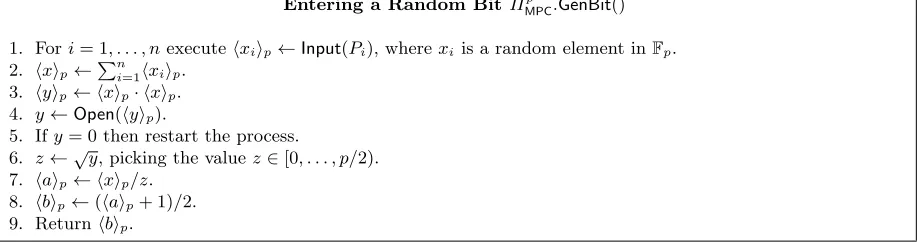
The main problem in performing actively secure key generation for SPDZ is to produce secure randomly shared bits within the MPC functionalities; in which the bit is zero with probability 1/2, and one with probability 1/2. The ‘standard’ trick to do this, borrowed from [11], for a single MPC functionality is given in Figure 45. However, if we execute this
procedure with respect to both FMPCp0 and FMPCp1 then we will obtain two shared random bits hb0ip0 and hb1ip1 but we will not necessarily haveb0 =b1.
To obtain shared random bits in the two MPC systems which are identical we need to adapt the daBit idea from [29]. In this paper it is shown how to obtain identical shared random bits in two MPC systems; one being a SPDZ-like system modulo p, and one being a BDOZ-like system over F2 based on OT for garbled circuit style computations. In our
key generation protocol we require shared random bits in two SDPZ-like systems for large moduli p0 and p1. This makes the protocol to generate the shared random bits a little easier
to understand than the one considered in [29]. Indeed we present a more general protocol than that which is needed for our key generation method. Our new method includes the case considered in [29], and is more efficient than the improved method considered in [3].
For our generalisation we consider a set of t SPDZ-like MPC systems with moduli
p0, . . . , pt−1. Our goal is to generate shares hbipi in all of these systems where b ∈ {0,1}.
5 If the underlying MPC system is SPDZ based then a more efficient way to perform the method is using the FHE
Entering a Random Bit ΠMPCp .GenBit()
1. Fori= 1, . . . , nexecutehxiip←Input(Pi), wherexi is a random element inFp. 2. hxip←Pni=1hxiip.
3. hyip← hxip· hxip. 4. y←Open(hyip).
5. Ify= 0 then restart the process.
6. z←√y, picking the valuez∈[0, . . . , p/2). 7. haip← hxip/z.
8. hbip←(haip+ 1)/2. 9. Returnhbip.
Figure 4.‘Standard’ method to produce a shared random bit inΠMPCp
Our method makes no restriction on the size of the primespi, nor the underlying SPDZ-like
MPC engine, thus our method can be used as a replacement for the daBit methods in [3,29] as well.
We definepmin to bemin(p1, . . . , pt) and we letγ be the smallest integer such thatpγmin>
2sec, where sec is our security parameter. For efficiency we will generate these shared bits in
batches of m at a time. We define an auxiliary prime number p which satisfies
p >(m+γ·sec)·2sec.
The prime p can be the same as one of the primes pi above. All we require is that the
MPC functionality FMPCp is extended by a command which we model via the ideal func-tionality FMPCp .GenBit() given in Figure 5. A protocol for BDOZ and MASCOT-SPDZ for FMPCp .GenBit() is given in Figure 4, with the equivalent SPDZ protocol satisfying the same ideal functionality, see for example [11].
FunctionalityFMPCp .GenBit()
1. For each corrupt partyPi, the functionality waits for inputsbi∈Fp.
2. The functionality waits for a messageabortorokfrom the adversary. If the message isokthen it continues. 3. The functionality then samples a bitb∈ {0,1}and the completes the sharing tob=P
biby selecting shares for the honest parties.
4. The (authenticated) shares are passed to the honest players. 5. The bitbis stored in the functionalityFMPCp .
Figure 5.The ideal functionality for single random bits
Our protocol will make use of the following result
Lemma 3.1. Let xi ∈[0, . . . , p) be such that
x1+. . .+xn=
k·p, or
k·p+ 1.
set ∆=dp/ne and write xi =li +∆·hi with 0≤li < ∆, then
k =l∆·
P
hi
p
m
with probability at least 1−1/p.
Proof. We have, for∈ {0,1},
k = ∆·
P hi p + P li p − p.
We have 0≤P
li < pby construction, and so the equality onkwill follow as long as P
li ≥.
But this always happens unless = 1 andP
li = 0, which happens with probability 1/p. ut
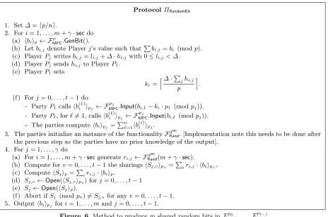
In Figure 6 we explain our protocolΠRandomBitfor producing shared random bits in the two
MPC systems. Intuitively the protocol works as follows. The parties generateM+γ·secshared random bits in the MPC engine FMPCp using the commandGenBit. They then determine the associatedk value for each shared bit using Lemma 3.1, this does not reveal any information about the hidden bit, but clearly reveals some (unimportant) information about the sharing6. Thinking of the sharing now as over the integers, and then reducing modulopi, PlayerP1 can
adjust his sharing so that the bit is correctly shared modulo pi. These shares are then input
into the MPC engines Fpi
MPC. Assuming all parties are honest we now have a valid sharing.
Protocol ΠRandomBit
1. Set∆=dp/ne.
2. Fori= 1, . . . , m+γ·secdo (a) hbiip← FMPCp .GenBit().
(b) Letbi,j denote Playerj’s value such thatPbi,j=bi (modp). (c) PlayerPj writesbi,j=li,j+∆·hi,j with 0≤li,j< ∆. (d) PlayerPj sendshi,j to PlayerP1.
(e) PlayerP1 sets
ki=
l∆· P
jhi,j p
m
.
(f) Forj= 0, . . . , t−1 do - PartyP1callshb(1)i ipj ← F
pj
MPC.Input(bi,1−ki·p1 (modpj)).
- PartyP`, for`6= 1, callshb(i`)ipj ← F
pj
MPC.Input(bi,` (modpj)).
- The parties computehbiipj =
Pn `=1hb
(`)
i ipj.
3. The parties initialize an instance of the functionalityF2sec
Rand. [Implementation note this needs to be done after
the previous step so the parties have no prior knowledge of the output]. 4. Forj= 1, . . . , γdo
(a) Fori= 1, . . . , m+γ·secgenerateri,j← F2
sec
Rand(m+γ·sec).
(b) Compute forv= 0, . . . , t−1 the sharingshSj,vipv =
P
iri,j· hbiipv.
(c) ComputehSjip=Piri,j· hbiip.
(d) Sj,v←Open(hSj,vipv) forj= 0, . . . , t−1
(e) Sj←Open(hSjip).
(f) Abort ifSj (modpv)6=Sj,vfor anyv= 0, . . . , t−1. 5. Outputhbiipj fori= 1, . . . , mandj= 0, . . . , t−1.
Figure 6.Method to producemshared random bits inFp0
MPC, . . . ,F
pt−1
MPC
6 In our security proof this information can be perfectly simulated by the simulator, and leaks no information about
To cope with dishonest parties we check the parties are honest by verifying random linear combinations. Here we note that the initial sharing inFMPCp is guaranteed to be a sharing of a bit due to the active security of the operation GenBit in FMPCp . Opening a random linear combination S of the shared bits in FMPCp is then a subset-sum over the integers, due to the lower bound on p. We then compare this to the associated sum modulo pi obtained from
Fpi
MPC. This has to be repeatedγ times to cope with the smallest value ofpi. We thus obtain
an instance of the Multiple-Subset-Sum-Problem (MSSP) considered in [27].
The protocolFMPCp .GenBit() in Figure 4 requires one secure multiplication and two rounds of communication (as a multiplication also requires a round of communication). To execute the rest of ΠRandomBit requires four rounds of communication (one for the initial opening
to P1, one for input into the MPC engines, one for executing F2
sec
Rand and one for the final
opening). If the m+γ·sec bits required inΠRandomBit are produced in parallel, as well as the
various input/open operations etc, this means that protocol ΠRandomBit requires
m+γ·sec
secure multiplications in FMPCp and 2 + 4 = 6 rounds of communication.
3.1 Multiple Subset Sum Problem
Definition 3.1 (Multiple Subset Sum Problem [27]). The MSSP is the problem of
given weights ai,j ∈Z>0 for i= 1, . . . , k and j = 1, . . . , n and target values s1, . . . , sk ∈Z to
find values xi ∈ {0,1} such that n X
j=1
ai,j ·xj =si for i= 1, . . . , k.
Just as the single subset-sum problem has a notion of density, for which one can trivially find solutions, the MSSP also has a notion of density. We define the density of an MSSP to be
d= n
k·max logai,j
.
We then have
Lemma 3.2 ([27]). If d < 0.9408 then the MSSP problem can ‘almost always’ be solved
with a single call to a lattice oracle.
In this work we restrict to MSSP problems with high density, i.e.d >1. In our protocol even if we set m = 1 the density of the subset sums S over the integers, which are revealed, is given by
d= 1 +γ·sec
γ·sec >1.
that even in the presence of malicious players the output is correct (i.e. m shared bits are the same in all Fpj
MPC). The main potential leakage of information comes from the opened
subset sum values over the integers, i.e.S. To deal with this leaked information we consider the following variant of the subset sum problem.
Definition 3.2 (Multiple Subset-Sum Guessing Problem (MSSG Problem)).Given
a set of random weights wi,j ∈ [0, . . . ,2γ·sec) for i = 1, . . . , v with v = γ · sec + 1 and
j = 1, . . . , γ, define mj = miniwi,j and sj = P
iwi,j. The problem is to distinguish between
the two different distributions:
1. In the first distribution the challenger picks random bits bi ∈ {0,1} and sets Sj = P
ibi·
wi,j. The values (S1, . . . , Sγ) are returned to the adversary. We write this as {Sj} ←D1.
2. In the second distribution the challenger samples values Sj ∈ [mj, . . . , sj] uniformly at
random and returns it to the adversary. We write this as {Sj} ←D2.
If A is an adversary then we define the advantage of A in solving this problem by
AdvA = 2· Pr
h
A( {wi,j}, {Sj} ) =b | b ← {1,2},
wi,j ←wi,j ∈[0, . . . ,2γ·sec),
Sj ←Db i
−1/2 .
We say the problem is hard if AdvA is a negligible function of sec for all polynomial time adversaries A.
We first discuss this problem. The condition v = γ ·sec+ 1 implies that the MSSP in the first distribution is not a low density multiple subset sum, and thus (if sec is chosen large enough) the underlying subset sum problem is hard.
There are approximately (v −1)·2γ·sec elements in the range [mj, . . . , sj], but only at
most 2v = 2γ·sec+1 of these correspond to valid subset sums. Thus the probability, in the
second distribution, that a random valueSj ∈[mj, . . . , sj] corresponds to a valid subset sum
is bounded above by
2γ·sec+1
(v−1)·2γ·sec ≈
2
v−1 =
2
γ·sec.
If we set sec = 128 then there is a 1/(γ · 64)γ chance that an instance selected by the second distribution is one which can be selected by the first distribution. This means that the advantage is not necessarily bounded by one for a perfect adversary.
To see this consider an adversary against the above problem, which outputs 1 if they believe the first distribution is what was sampled from and 2 if they believe it is the second. If they always output the first distribution then they are correct with probability 1/2, if they always output the second distribution then they are also correct with probability 1/2. Thus zero advantage still corresponds to an adversary which makes no intelligent choices at all.
have a problem when they deduce distribution D1 since this distribution could have arisen
by chance from a challenger selection of b = 2 probability 1/64γ. Thus for this adversary
(supposedly perfect adversary) we have
AdvA= 2·
1
2 ·( Pr[ A(. . .) = 1 | b= 1 ] + Pr[ A(. . .) = 2 | b = 2 ] )− 1 2
= (1 + (1−1/64γ)−1) = 1− 1 64γ.
We finally note that the best algorithms for the subset-sum problem, on elements of size
V = 2sec, have time either O(2sec/2) [18] or O(sec·2sec) [28], or O(V ·√sec) [24]. With our parameters, these all have exponential time as V = 2sec.
3.2 Security of ΠRandomBit
We now discuss the security of this protocol. Formally we want the protocol to extend the pair of functionalities (FMPCp0 , . . . ,Fpt
MPC), with the procedure defined in Figure 7. The
functionalityFRandomBits internally generates a set of msecure bits, and we require that even
if some information about these bits is leaked to the adversary that the remaining bits are still secure. We need this additional leaking of a subset of bits, as we do not know how the secure bits will be used in any following MPC protocol, thus we must assume the worst that a subset leaks. Even if m−1 bits are revealed or some information about them is leaked then we want the final remaining bit to still be secret.
FunctionalityFRandomBits
1. Fori= 1, . . . , m+γ·secthe functionality callsFp
MPC.GenBit() so as to store a bitbi. 2. The bitsbiare retrieved fromFMPCp and are enterred into the functionalitiesF
pj
MPCforj= 0, . . . , t−1.
3. The functionality waits for a messageabortorokfrom the adversary. If the message isokthen it continues. 4. The functionality waits for a proper subsetS of{1, . . . , m}from the adversary and returns the bitsbj for j ∈ S to the adversary. [We note this subset can be adaptively chosen, but to simplify the exposition we assume it is presented to the functionality in one go.]
Figure 7.The ideal functionality for random bits
Theorem 3.1. Assume the problem Multiple Subset Sum Guessing (MSSG Problem) is
hard then protocolΠRandomBit securely implements FRandomBits in theF2
sec
Rand,FMPC. GenBit-hybrid
model.
Proof. The valuesSj are produced with no wrap-around modulop, due to the bound onM.
Thus the γ values Sj define subset sums over the integers
Sj =
M+γ·sec X
i=1
where we are guaranteed that bi ∈ {0,1}.
We then check these sums against the equivalent sums modulo pv for v = 0, . . . , t−1.
Since the random coefficients ri,j are revealed only after the parties input their shares b (p) i
of the bits modulo pv, the fact that the values Sj,v are equal to Sj (mod pv) implies with
overwhelming probability (since pγmin > 2sec) that the shared values entered modulo p j are
equal to the shared values in FMPCp .
Since FMPCp .GenBit generates values which are gauranteed to be bits, this implies the values modulo pj are also bits, and equal to each other.
To complete the proof we must show that the protocol can be simulated. There are two sets of values which need simulating. Thehi,j values which are sent to partyP1 by PlayerPj
and the subset sum values Sj and Sj,v which are opened. We first deal with the hi,j values.
The simulator already knows the shares hi,j which the adversary should be sending to
them (fromFMPCp .GenBit), and so knows whether to abort the functionality at this point. To generate the hi,j values for the honest parties the simulator simply picks random values for
the honest parties shares bi,j so that they sum to zero modulo p. The honest hi,j are then
derived from these values. These top bits of the honest shares will be a valid simulation even if the shared bit is actually one.
To simulate the value Sj, and hence Sj,v, we simply define the trivial simulator. The
values ri,j are sampled using the ideal functionality F2
sec
Rand, and then the valuesmj =min ri,j
and sj = P
ri,j are computed. It then picks a random valueSj ∈[mj, . . . , sj] and returnsSj
and Sj,v =Sj (mod pv), for every v, to the adversary. When the adversary selects a proper
subset S of {1, . . . , m} to be opened, it queries the ideal functionality and returns these values.
We now show that an environment that can distinguish between a real-world execution and the ideal-world execution with this simulator can be used to solve an arbitrary instance of the MSSG problem. We let A denote our adversary against the MSSG problem. This takes as input t = sec + 1 values w1,j, . . . , wt,j, for j = 1, . . . , γ, and a target sum Tj for
j = 1, . . . , γ. The adversary A runs the environment twice as follows, where we let the run be denoted by the variable r∈ {1,2}.
1. The adversary A selects an index i∗r ∈ {1, . . . , m}. 2. The adversary setsri(r)∗
r,j to bewt,j.
3. The adversary setsri+m,j(r) =wi,j for i= 1, . . . ,sec.
4. The adversary selects all other valuesri,j(r), for runr, at random from [0, . . . ,2sec). 5. For i∈ {1, . . . , m} \ {i∗r} the adversary selects a bit b(r)i ∈ {0,1}.
6. The adversary sets Sj(r) =Tj + P
b(r)i ·r(r)i,j, where the sum is overi∈ {1, . . . , m} \ {i∗r}. 7. The adversary then runs the environment, revealing the valuesSj(r), andSj(r) (mod pv) as
required.
8. At some point the environment in runr will request a subset of queries Sr ⊂ {1, . . . , M}.
At this point for every i ∈ Sr the adversary returns b (r)
i if i 6= i
∗
r. If i = i
∗
r then the
10. In the case of a value returned of real in either run, the adversary A decides its input problem was from the first MSSG distribution.
11. Otherwise the adversary decides that its input was from the second MSSG distribution. We now discuss why this adversary solves the MSSG problem. Notice that if i∗r 6∈ Sr for one
of the two executions, then this execution is indistinguishable by definition to the real world execution when the input problem is from the first MSSG distribution and is equal to the ideal world execution when the input problem is from the second MSSG distribution.
When i∗r ∈ Sr, and the input problem is from the first MSSG distribution, and the bit
corresponding to this solution is correct (i.e. is actually equal to r−1) then the adversary is presenting an execution indistinguishable from the real world. If the bit is wrong, i.e. not equal to r−1, then the execution is unlikely to be identical to a real execution (unless there is a solution to the subset sum with b(r)i∗
r equal to 2−r). Since we run the adversary twice in such a case we are guaranteed that if the input is from the first MSSG distribution one of our executions will be correctly equal to the real distribution.
In the case wheni∗r ∈ Sr for both values ofr and the input distribution to A is from the
second MSSG distribution, then the view given to the distinguisher is that of the simulated distribution.
Thus in all cases any distinguisher which can distinguish between the real and ideal world
will be able to be used by A to solve the MSSG problem. ut
As pointed out to us by Carsten Baum we can remove the need to assume our variant of the subset-sum protocol in the above theorem if we increase the number size of our subset sum from m+γ·sec tom+ 2·γ·sec. This obviously reduces the efficieny of the protocol. If one is willing to pay this price then security becomes a purely statistical argument. Such an argument is similar to arguments used in prior works in various situations, see for example [21,30].
4
Sampling Distributions In MPC
In this section we explain how we perform the various sampling operations we need in the key generation algorithm. We assume that two actively-secure (with-abort) MPC functionalities, as in Figure 2, have already been initiated, one for the primep0 and one for the primep1. We
call these two functionalitiesFMPCp0 and FMPCp1 . As explained earlier these can be instantiated with either BDOZ or MASCOT-SPDZ. Using these functionalities we instantiate the protocol
ΠRandomBit, from Section 3, to produce doubly-authenticated bits in both FMPCp0 and FMPCp1 .
The protocol ΠHamming will only be used to generate secret keys which are equivalent
to the traditional BGV style keys used in SCALE-MAMBA or HELib. For more modern implementations one will use ΠBinomial to generate the secret keys as these have less security
concerns related to them. In both cases we need ΠBinomial and ΠUniform to generate the error
vectors needed to compute the public key.
Additionally we see our ΠHamming protocols family could potentially improve the cost of
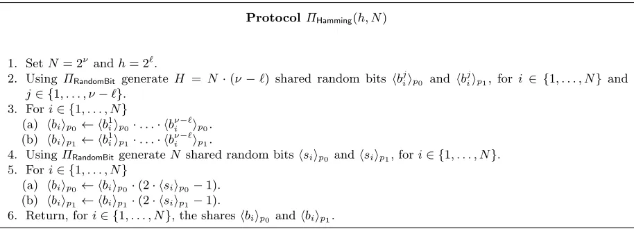
4.1 Protocol ΠHamming
To sample our secret key we will need to sample a shared vector of length N, with elements in {−1,0,1}, with approximate Hamming weight h, i.e. we sample from B(h/N)N. The
values of N and h are selected such they are both powers of two, so we set N = 2ν and
h = 2`. The reader should think of values of N = 32768 and h = 64, which are used in
SCALE-MAMBA’s default configuration. To sample such vectors we use protocolΠHamming(h, N)
given in Figure 8.
Protocol ΠHamming(h, N)
1. SetN= 2νandh= 2`.
2. Using ΠRandomBit generate H = N·(ν−`) shared random bits hbjiip0 and hb
j
iip1, for i ∈ {1, . . . , N} and
j∈ {1, . . . , ν−`}. 3. Fori∈ {1, . . . , N}
(a) hbiip0← hb 1
iip0·. . .· hb
ν−` i ip0.
(b) hbiip1← hb 1
iip1·. . .· hb
ν−` i ip1.
4. UsingΠRandomBitgenerateN shared random bitshsiip0 andhsiip1, fori∈ {1, . . . , N}.
5. Fori∈ {1, . . . , N}
(a) hbiip0← hbiip0·(2· hsiip0−1).
(b) hbiip1← hbiip1·(2· hsiip1−1).
6. Return, fori∈ {1, . . . , N}, the shareshbiip0 andhbiip1.
Figure 8.Method to produce vectors of (expected) Hamming weighthwith elements in{−1,0,1}
We again estimate the cost of this operation. If we assume that the two calls toΠRandomBit
require only one batch operation then these operation requires 6 rounds of communication, (H+N +sec) multiplications in FMPCp 7. The products to produce the initial bits b
i require
dlog2(ν−`)e rounds of communication and (ν −` −1)·N multiplications in both FMPCp0 and FMPCp1 . Whereas the products to produce the final signed bits require one round of communication and N multiplications in both FMPCp0 and FMPCp1 . Hence in total we require
6 +dlog2(ν−`)e+ 1 = 7 +dlog2(ν−`)e rounds of communication and
NHamming,0 =N +H+sec+ (ν−`+ 1)·N,
NHamming,1 = (ν−`+ 1)·N
total multiplications in ΠMPCp0 and ΠMPCp1 respectively.
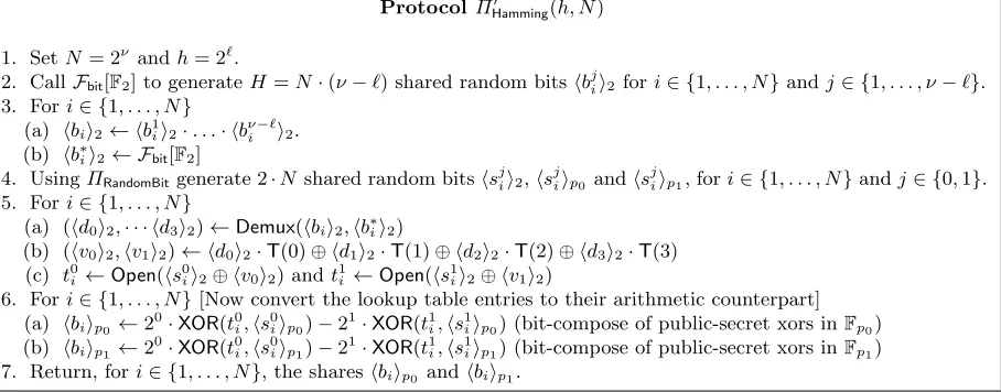
4.2 Another Method to Implement ΠHamming
In this section we describe a different protocol to generate a vector of size N with expected hamming weight h. The main advantage of this protocol is that it avoids the expensive mul-tiplications modulo large prime numbers (modulop0 and modulop1) completely. This comes
7
at the expense of requiring an extra preprocessing protocol which generates random shared bits modulo two from [21,30], as well as the need to implement a demultiplexer via a lookup table [20]. Thus this method requires us to base the SPDZ key generation methodology on two distinct MPC methodoligies; TinyOT-styleF2-based MPC and MASCOT style Fp-base
MPC. So as to keep the minimality in terms of base MPC protocols for our key generation process we include this section mearly as an additional method for the reader.
Note that to generate random bits shared modulo two is much cheaper than generating random shared bits modulo a large prime p. These binary sharings are usually done using a pairwise protocol TinyOT style found in Wang et al. or Keller et al. [21,30]. We call the functionality that generates binary sharings Fbit[F2]
The key idea of this protocol is to follow the same blueprint as ΠHamming(h, N) defined in
Section 4.1 but start with random binary sharings of bitshbi2 rather then arithmetic sharings
hbip0 andhbip1. This will cause the bit multiplications to happen modulo two which is orders
of magnitude faster than their counterpart modulo a large primep.
However, the main challenge with this method is to be able to output the value in {0,±1} without the large field multiplications in Step 5 from Figure 4.1. This can be done by emulating a small demultiplexer on the values bib∗i ({00,01,10,11}) and map them to
{0,0,1,−1}. We define this public lookup table containing these values in binary form as
T={00,00,10,11}. One can think of the last bit in each entry of Tas the sign of the secret key bit. In the last step we convert the table entries to integers modulo a large prime using maBits, i.e. compute 20·T(i, j)−21·T(i, j) where T(i, j) represents the j’th bit of the i’th
entry.
Protocol ΠHamming0 (h, N)
1. SetN= 2νandh= 2`.
2. CallFbit[F2] to generateH=N·(ν−`) shared random bitshbjii2 fori∈ {1, . . . , N}andj∈ {1, . . . , ν−`}.
3. Fori∈ {1, . . . , N}
(a) hbii2← hb1ii2·. . .· hbνi−`i2.
(b) hb∗
ii2← Fbit[F2]
4. UsingΠRandomBitgenerate 2·N shared random bitshsjii2,hsjiip0 andhs
j
iip1, fori∈ {1, . . . , N}andj∈ {0,1}.
5. Fori∈ {1, . . . , N}
(a) (hd0i2,· · · hd3i2)←Demux(hbii2,hb∗ii2)
(b) (hv0i2,hv1i2)← hd0i2·T(0)⊕ hd1i2·T(1)⊕ hd2i2·T(2)⊕ hd3i2·T(3)
(c) t0
i ←Open(hs0ii2⊕ hv0i2) andt1i ←Open(hs1ii2⊕ hv1i2)
6. Fori∈ {1, . . . , N}[Now convert the lookup table entries to their arithmetic counterpart] (a) hbiip0←2
0·XOR(t0
i,hs0iip0)−2
1·XOR(t1
i,hs1iip0) (bit-compose of public-secret xors inFp0)
(b) hbiip1←2 0·
XOR(t0i,hs0iip1)−2 1·
XOR(t1i,hs1iip1) (bit-compose of public-secret xors inFp1)
7. Return, fori∈ {1, . . . , N}, the shareshbiip0 andhbiip1.
Figure 9.Second method to produce vectors of (expected) Hamming weighthwith elements in{−1,0,1}
4.3 Protocol ΠBinomial
The protocol for sampling shared values from the distributiondN(σ2, N) is relatively
pro-tocol consists entirely of linear operations. Thus the round complexity is six and it requies
NBinomial= 2·k·N+sec multiplications in FMPCp .
Protocol ΠBinomial(σ2, N)
1. Definekbyσ=pk/2.
2. UsingΠRandomBitgenerate 2·k·N shared random bitshbjiip0 andhb
j
iip1, fori∈ {1, . . . , N}andj∈ {0, . . . ,2·
k−1}.
3. Fori∈ {1, . . . , N} (a) hbiip0←
Pk−1
j=0hb 2·j i ip0− hb
2·j+1
i ip0.
(b) hbiip1←
Pk−1
j=0hb 2·j i ip1− hb
2·j+1
i ip1.
4. Return, fori∈ {1, . . . , N}, the shareshbiip0 andhbiip1.
Figure 10.Method to produce elements fromdN(σ2, N)
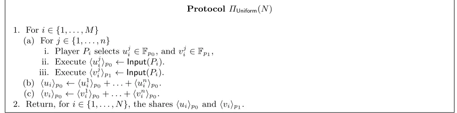
4.4 Protocol ΠUniform
Our final protocol is a rather trivial one, it allows the parties to sample a uniform element fromZq in a secret shared form, we give it in Figure 11.
ProtocolΠUniform(N)
1. Fori∈ {1, . . . , M} (a) Forj∈ {1, . . . , n}
i. PlayerPiselectsuji ∈Fp0, andv
j i ∈Fp1,
ii. Executehujiip0 ←Input(Pi).
iii. Executehvj
iip1 ←Input(Pi).
(b) huiip0← hu 1
iip0+. . .+hu
n iip0.
(c) hviip0← hv 1
iip0+. . .+hv
n iip0.
2. Return, fori∈ {1, . . . , N}, the shareshuiip0 andhviip1.
Figure 11.Protocol to sample a uniform element fromZq
5
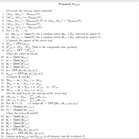
SPDZ KeyGeneration
Given the previous algorithms to generate various distributions the computation of the actual key generation algorithm becomes relatively straight forward. We first sample the various distributions modulo p0 and p1, then we produce the square of the secret key (needed for
the key switching matrices), and then we output the public key and recombine it using the CRT, then we do the same to each players component of the secret key. The overall protocol is given in Figure 12; note that in line 3 one can select as to whether to choose the secret key from a restricted Hamming weight or from the centred binomial distribution. To make the protocol easier to follow we use the notation haip0 etc to denote a vector of N shares
We let haip0 hbip0 denote the multiplication of two such vectors when considered as
elements in the ring Rp0. This requires one round of communication and N2 secure
multi-plications (or N ·(N −1)/2 secure multiplications if a = b). If one vector is in the clear then we write a hbip0, which is a linear operation and hence for “free”. A more efficient
method to multiply is to use the FFTalgorithm, which recall is a linear operation and thus ‘free’ when executed in the MPC engine. To multiply using FFT we utilize
haip0 hbip0 =FFT−1(FFT(haip0)·FFT(hbip0)
which requires only N secure multiplications and one round of communication.
We now examine each of the operations in this algorithm in turn. The lines 1-6 can all be executed in parallel and so require
max6 +dlog2(ν−`)e+ 1,6,1= 6 +dlog2(ν−`)e
rounds of communication8 in the case where we select restricted Hamming weight secret key
and
max
6,6,1
= 6
for the case of the secret key generated from a centred binomial distribution. The number of secure multiplications is given by, in the two cases,
NHamming,0+NHamming,1 + 2·NBinomial=N +H+sec+ 2·(ν−`+ 2·k−1)·N,
3·NBinomial= 6·k·N.
Lines 7 and 9 are linear operations and thus can be executed as purely local operations. Line 8 requires one round of communication andN multiplications inFMPCp0 . Note, in lines 7-9 we only have to compute sk2 modulo p0 as it is multiplied by p1 when added into bsk,sk2. Lines 10-13 can also be performed in parallel and hence require only one round of communication. The lines 16-21 are all local operations, and hence are for “free”. Lines 25-24 are, again, able to be done in parallel and so require only one round of communication. The remaining lines are purely local organization of data into the correct format for outputing. Thus the total number of rounds of communication (assuming all shared random bits are produced in a single batch) is
12 +dlog2(ν−`)e or 12 depending on which variant one is using for the secret key.
If we take typical values of n = 2, N = 32768, h = 64, and sec = 128 then these work out to be 3277056 mults in ΠMPCp0 and 3244288 in ΠMPCp1 and 16 rounds of communication.
Theorem 5.1. The protocolΠKeyGen UC-securely realises the functionalityFKeyGen against a
static, active adversary corrupting at mostn−1parties in the FMPCp -hybrid model, assuming the decision subset-sum problem is hard.
8 Of course in practice we generate the secure bits in batches and hence this is just the minimal number of rounds
Protocol ΠKeyGen
- [Generate the various values required] 1. (haip0,haip1)←ΠUniform(N).
2. (ha0ip0,ha 0
ip1)←ΠUniform(N).
3. (hsip0,hsip1)←ΠHamming(h, N) or (hsip0,hsip1)←ΠBinomial(N).
4. (heip0,heip1)←ΠBinomial(N).
5. (he0i
p0,he 0i
p1)←ΠBinomial(N).
6. Fori∈ {2, . . . , n}
(a) hsk0,iip0←Input(Pi) for a random vectorsk0,i∈Rp0 selected by playerPi.
(b) hsk1,iip1←Input(Pi) for a random vectorsk1,i∈Rp1 selected by playerPi.
- [Compute the square of the secret key] 7. hfip0 ←FFT(hsip0).
8. hf0ip0 ← hfip0· hfip0 [This is the component wise product].
9. hs0i
p0←FFT −1(hf0i
p0).
- [Open the valuesaanda0] 10. a0←Open(haip0).
11. a1←Open(haip1).
12. a00←Open(ha0ip0).
13. a01←Open(ha 0i
p1).
14. a←CRT([a0,a1],[p0, p1]).
15. ask,sk2←CRT([a00,a01],[p0, p1]).
- [Computebandb0]
16. hbip0←a0 hsip0+p· heip0.
17. hbip1←a1 hsip1+p· heip1.
18. hb0i
p0←a 0
0 hsip0+p· he 0i
p0−p1· hs 0i
p0.
19. hb0i
p1←a 0
1 hsip1+p· he 0i
p1.
- [Fix the final key for the sharing of the secret key] 20. hsk0,1ip0← hsip0−
Pn
i=2hsk0,iip0.
21. hsk1,1ip1← hsip1−
Pn
i=2hsk1,iip1.
22. For alli∈ {1, . . . , n}assignski←CRT([sk0,i,sk1,i],[p0, p1]).
23. P1←Output(hsk0,1ip0).
24. P1←Output(hsk1,1ip1).
- [Open the valuesbandb0] 25. b0←Open(hbip0).
26. b1←Open(hbip1).
27. b00←Open(hb 0
ip0).
28. b01←Open(hb0ip1).
29. b←CRT([b0,b1],[p0, p1]).
30. bsk,sk2←CRT([b00,b01],[p0, p1]).
31. Outputa,b,ask,sk2 andbsk,sk2 to all players, andskito playerPi.
Proof. We define the simulatorS as follows. The simulator emulates the behaviour of honest parties exactly, but additionally does the following:
- At the start of the execution, the simulator initialises a local copy of FMPCp0 and FMPCp1 and sends the message start to FKeyGen and awaits the public key pk = (¯a,b,¯ ask¯,sk2,bsk¯,sk2) in
response.
- When the adversary and simulator execute ΠUniform, the simulator replaces the values a
mod p0, a modp1, a0 mod p0 and a0 mod p1 stored in the instances of FMPCp0 and F p1 MPC,
respectively, with ¯a modp0, ¯a modp1, ask¯,sk2 mod p0 and ask¯,sk2 mod p1.
- In Step 6, for each j ∈ [n], if j is corrupt and j > 2 then the simulator awaits the input
skj,0 and skj,1 for each corrupt party Pj and constructs skj ← CRT(skj,0,skj,1), and sends
these toFKeyGen.
- Just before opening b0, b1, b00 and b
0
1 the simulator replaces these values stored in the
instances ofFMPCp0 andFMPCp1 with ¯b mod p0, ¯b mod p1,bsk¯,sk2 mod p0andbsk¯,sk2 modp1.
Since the only inputs to the protocol are randomly sampled by parties, the simulator can perfectly emulate the behaviour of honest parties throughout, as the environment does not observe the random tape of honest parties or the simulator. Indeed, since FMPCp0 and FMPCp1 are used as black boxes and the only communication between parties occurs via these functionalities, which are emulated locally honestly by the simulator, the replacements made in the simulation outlined are executed without being observed by the environment (at this point). Moreover, the inputs of corrupt parties can be extracted trivially and passed on to FKeyGen so that the final outputs have the correct distribution.
It only remains to show that the environment cannot observe a difference between the transcripts in a real execution and an execution in which the replacements described above are made. While the final outputs of the real and ideal worlds is the same, the distribution of the transcript differs since communication generated in the execution of the sampling subprotocols depends on the secret ¯s which is (implicitly) generated by the functionality FKeyGen when executingKeyGen() and cannot be computed by the simulator from the public
key without breaking the LWE assumption for the security of the key. We must show that the amount by which the distributions differ is negligible.
The only time information stored in FMPCp0 or FMPCp1 is either revealed to the parties or is generated by parties is in the bits shared in ΠRandomBits and in ΠUniform. In the protocols
ΠBinomial and ΠHamming the parties obtain bits from ΠRandomBits, and in the remainder of the
protocol ΠKeyGen, the correctness of the computations is guaranteed by the security of the
black boxes FMPCp0 and FMPCp1 . In ΠUniform, every party contributes to every secret, and since
there is at least one honest party (that samples uniformly), the output is always uniform. Thus it suffices to argue that nothing can be learnt in ΠRandomBits about the bits that are
generated (which are later used to generate the public key) without solving the subset sum problem. But this follows from Theorem 3.1. Thus no distinguishing environment can exist, by the choice of parameters for the subset sum, and therefore ΠKeyGen UC-securely realises
6
Implementation
In our implementation we use MASCOT [22] as the base protocol used for our one-time setup phase for SPDZ. We could have selected here BDOZ [5] using LowGear [23] for the pre-processing. Both giveO(n2) protocols with LowGear about a factor of four times faster for
small values ofn. Since our solution is built on top of theSCALE-MAMBA[2] framework, we re-used a lot of their already existing codebase and hence selected MASCOT as the underlying protocol. As explained in the introduction our key generation protocol, is inherently O(n2)
in nature. This seems to be unavoidable as the only practical O(n) MPC protocol known is SPDZ, which is exactly the MPC protocol we are trying to instantiate with our key generation protocol.
Selection of FHE parameters We recall that the two-leveled BGV key generation
proce-dure requires us to choose two prime moduli p0 and p1 and a polynomial degree N to define
the ciphertext space Rq ∼= Rp0 ×Rp1 and a prime p which defines the size of our plaintext
space. In addition we require that the relations presented in 2.2 hold.
The size of the plaintext space p defines the modulus of the underlying secret sharing scheme in the SPDZ protocol. Different values of p will be needed for different application scenarios. In this paper we focus on p ≈ 264 and p ≈ 2128. The precise sizes of the other parameters are derived from a noise analysis of how the resulting encryption scheme is used, which takes into account the circuit being computed, the zero-knowledge proofs required, and the distributed decryption procedure, and the computational difficulty of the Ring-LWE problem. This analysis is quite involved and we referred to theSCALE-MAMBAdocumentation [2] to obtain the required parameters.
This gives us (for example) that to guarantee a computational security of 128 bits with a polynomial degree N = 32768, our ciphertext modulus q has to verify q <2883. For such
parameters, the trusted setup of SCALE-MAMBA, as we have discussed earlier, produces a secret key with Hamming Weight exactly 64, and uses noise vectors distributed according to a centred binomial distribution with standard deviation of 3.16 = √10. As a first set of experiments we use exactly the same methodology to select the secret key, but we pick a secret key with expected Hamming Weight 64. This does not change the noise analysis (which is done using an expected noise methodology for the secret key in any case), and thus we end up with the same system parameters as used in SCALE-MAMBA. In particular for a plaintext modulus of 128 bits this leads us to use ap0 modulus of 345 bits and a p1 modulus
of 225 bits. So in order to run the key generation protocol presented above, we will need to run two instances of the MASCOT protocol; one for the 345 bits prime p0 and another for
the 225 bits primep1.
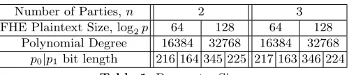
We tried different sets of parameters in our experiments, which provide BGV keys for a SPDZ modulus of 64 and 128 bits, always taking the same parameters as the Setup phase
for SCALE-MAMBA. In Table 1 we report the prime sizes, in bits, required for each set of
parameters for two and three parties.
Number of Parties,n 2 3 FHE Plaintext Size, log2p 64 128 64 128
Polynomial Degree 16384 32768 16384 32768 p0|p1 bit length 216 164 345 225 217 163 346 224
Table 1.Parameter Sizes.
the total number of shared bits that we will need, and also small enough to avoid RAM or network overflow. Empirically we found that taking 50000≤m≤100000 (depending on the setting) gives us good results.
Extended Random Oblivious Transfer: The SCALE-MAMBAframework does not have an
implementation of the offline phase of MASCOT, and an implementation of the extended Random Oblivious Transfer for a prime field Fp, thus we needed to implement these. The
triple generation method of MASCOT [22][Protocol 4] makes use of an extended Correlated Oblivious Transfer (COT) protocol. For this we used the passively secure protocol of Fred-eriksen et al. [14][Full Version, Figure 19] (which is essentially the protocol of Ishai et al [19]). Such a passively secure COT protocol is sufficient due to how it is used in the MASCOT offline phase. This COT protocol was already implemented in SCALE-MAMBA. For two parties
Pi and Pj with the former acting as the sender and the later as the receiver, calls to the
Correlated Oblivious Transfer output values{Mk
0, M1k =M0k+∆i}k∈[n] toPi and{Mbkk}k∈[n] to Pj, where ∆i ∈ F2128 is the input from Pi and b ∈ {0,1}n is the choice vector from Pj,
and ∀k ∈[n]Mk
0 ←$ F2128
To obtain extended Random Oblivious Transfer (ROT), from these extended COTs, we used the decorrelation technique presented in [8][Figure 15] which consists in both parties hashing the output of the extended COT. This gives us an extended ROT inF2128. However,
we want to run the MASCOT protocol on prime fields Fp0 and Fp1, so to translate our
extended ROT from F2128 to Fp, we take dlog2(p)+128
128 e outputs in F2128, concatenate them
together and take the result mod p.
Results of our experiments Our implementation of the key generation protocol was tested
in a LAN setting, with each party running on an Intel i7-7700K CPU with 32GB of RAM over a 10Gb/s network switch. In our experiments we found that executing more threads than the available number of cores (in our case eight) gave a performance improvement. This is because the computation between receiver and sender in the OT protocols is asymmetric, resulting in each party sometimes waiting for the other to perform some computation.
n 2 3
log2p 64 128 64 128
1 Thread 126.77 177.1 70.01 133.29 58.78 79.01 28.7 57.22 5 Thread 587.77 784.69 292.18 567.62 276.38 376.65 134.62 279.27 10 Thread 759.1 1032.57 365.93 740.05 389.19 547.27 185.32 379.34
Table 2.Triple Throughput forFp0 andFp1 in Triples per Second
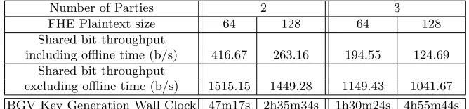
Finally in Table 3 we give figures related to the throughput of the secure randomly shared bits, namely the throughput of the algorithm in Figure 6, in the four different scenarios we experimented with. For each case, we give our result while also running the MASCOT triple generation, and also assuming that this offline phase has already been done beforehand. In the same table we eventually give the total runtime for the distributed BGV key generation procedure, which includes the time to perform the MASCOT offline phase.
Number of Parties 2 3
FHE Plaintext size 64 128 64 128
Shared bit throughput
including offline time (b/s) 416.67 263.16 194.55 124.69 Shared bit throughput
excluding offline time (b/s) 1515.15 1449.28 1149.43 1041.67
BGV Key Generation Wall Clock 47m17s 2h35m34s 1h30m24s 4h55m44s
Table 3.Shared bit throughput and total time for the KeyGen protocol.
We can observe that for two parties it takes between 47 minutes and five hours to complete the distributed key generation. Although it may seem inefficient, we argue that this protocol needs only to be done once in order to enable future computation of the offline phase of SPDZ. Moreover, we have shown that our protocol is highly parallelizable. So in practice, if such a protocol was to be run on high end servers owned by cloud service providers, the total runtime could be drastically reduced.
We pause to compare these run-times to the covertly secure distributed key generation protocol presented in [11]. This protocol did not produce public and secret keys with the same distribution as the non-distributed version. For plaintexts of 64-bits the authors of this paper report 12 and 16 seconds key generation time for n = 2 and n = 3, for a covert security of 1/10, i.e. an adversary can cheat with probability 1/10. For plaintexts of 128-bits the times are 33 and 44 seconds. The execution time of this covertly secure protocol is linear in c, where the covert security is 1/c. Thus to obtain comparable security to our protocol, the protocol in [11] would be utterly inpractical.
6.1 Changing the Standard Deviation
Table 1 is roughly the same. However, the associated run times for key generation become faster as we no longer need to generate as many doubly authenticated bits. This is reflected in Table 4. We see that by choosing σ = 0.707, we need only two bits instead of 40 for the sampling from the centred binomial distribution. We thus get a factor of at least 2.5 improvement over the previous setting.
Number of Parties 2 3
FHE Plaintext size 64 128 64 128
BGV Key Generation Wall Clock 16m10s 1h03m19s 28m46s 1h52m54s
Table 4.Shared bit throughput and total time for the KeyGen protocol forσ= 0.707.
6.2 Secret Keys Generated According to a Centred Binomial Distribution
Finally we examine the case of using the centred binomial distribution for generating the secret keys, with standard deviation selected to be σ = p1/2 = 0.707. This pushes the parameter sizes for the underlying BGV scheme up a little, as we need to cope with more potential noise growth due to the ‘heavier’ secret key. Using the same analysis as before we find the parameter sizes given in Table 5, with the resulting run times for distributed key generation given in Table 6. This time we performed the experiments also for n = 4 and n = 5 so as to show how the times grow with n; recall the overall method is O(n2) as
mentioned earlier.
Number of Parties,n 2 3 4 5 FHE Plaintext Size, log2p 64 128 64 128 64 128 64 128
Polynomial Degree 16384 32768 16384 32768 16384 32768 16384 32768
p0|p1 bit length 222 159 352 219 223 158 353 218 223 158 353 228 223 158 353 228
Table 5.Parameter Sizes for secret keys distributed according to a centred binomial distribution, and Gaussian error distribution ofσ= 0.707.
Number of Parties 2 3 4 5
FHE Plaintext size 64 128 64 128 64 128 64 128
BGV Key Generation 5m08s 18m20s 8m12s 26m35s 11m23s 52m48s 16m14s 2h11m42s
Acknowledgements
The authors would like to thank Carsten Baum and Emmanuela Orsini for suggestions in relation to the work in this paper. This work has been supported in part by ERC Ad-vanced Grant ERC-2015-AdG-IMPaCT, by the Defense AdAd-vanced Research Projects Agency (DARPA) and Space and Naval Warfare Systems Center, Pacific (SSC Pacific) under contract No. N66001-15-C-4070 and FA8750-19-C-0502, by the Office of the Director of National In-telligence (ODNI), InIn-telligence Advanced Research Projects Activity (IARPA) via Contract No. 2019-1902070006, by the FWO under an Odysseus project GOH9718N, and by Cyber-Security Research Flanders with reference number VR20192203. Any opinions, findings and conclusions or recommendations expressed in this material are those of the author(s) and do not necessarily reflect the views of the ERC, ODNI, United States Air Force, IARPA, DARPA, the US Government or FWO. The U.S. Government is authorized to reproduce and distribute reprints for governmental purposes notwithstanding any copyright annota-tion therein.
References
1. Alkim, E., Ducas, L., P¨oppelmann, T., Schwabe, P.: Post-quantum key exchange - A new hope. In: Holz, T., Savage, S. (eds.) USENIX Security 2016: 25th USENIX Security Symposium. pp. 327–343. USENIX Association, Austin, TX, USA (Aug 10–12, 2016)
2. Aly, A., Cozzo, D., Keller, M., Orsini, E., Rotaru, D., Scherer, O., Scholl, P., Smart, N.P., Wood, T.: SCALE-MAMBA v1.8: Documentation (2020),https://homes.esat.kuleuven.be/~nsmart/SCALE/Documentation.pdf 3. Aly, A., Orsini, E., Rotaru, D., Smart, N.P., Wood, T.: Zaphod: Efficiently combining LSSS and garbled circuits in SCALE. In: Brenner, M., Lepoint, T., Rohloff, K. (eds.) Proceedings of the 7th ACM Workshop on Encrypted Computing & Applied Homomorphic Cryptography, WAHC@CCS 2019, London, UK, November 11-15, 2019. pp. 33–44. ACM (2019),https://doi.org/10.1145/3338469.3358943
4. Asharov, G., Jain, A., Wichs, D.: Multiparty computation with low communication, computation and interaction via threshold FHE. Cryptology ePrint Archive, Report 2011/613 (2011),http://eprint.iacr.org/2011/613 5. Bendlin, R., Damg˚ard, I., Orlandi, C., Zakarias, S.: Semi-homomorphic encryption and multiparty computation.
In: Paterson, K.G. (ed.) Advances in Cryptology – EUROCRYPT 2011. Lecture Notes in Computer Science, vol. 6632, pp. 169–188. Springer, Heidelberg, Germany, Tallinn, Estonia (May 15–19, 2011)
6. Boyle, E., Couteau, G., Gilboa, N., Ishai, Y., Kohl, L., Scholl, P.: Efficient pseudorandom correlation generators: Silent OT extension and more. In: Boldyreva, A., Micciancio, D. (eds.) Advances in Cryptology – CRYPTO 2019, Part III. Lecture Notes in Computer Science, vol. 11694, pp. 489–518. Springer, Heidelberg, Germany, Santa Barbara, CA, USA (Aug 18–22, 2019)
7. Brakerski, Z., Gentry, C., Vaikuntanathan, V.: (Leveled) fully homomorphic encryption without bootstrapping. In: Goldwasser, S. (ed.) ITCS 2012: 3rd Innovations in Theoretical Computer Science. pp. 309–325. Association for Computing Machinery, Cambridge, MA, USA (Jan 8–10, 2012)
8. Burra, S.S., Larraia, E., Nielsen, J.B., Nordholt, P.S., Orlandi, C., Orsini, E., Scholl, P., Smart, N.P.: High performance multi-party computation for binary circuits based on oblivious transfer. Cryptology ePrint Archive, Report 2015/472 (2015),http://eprint.iacr.org/2015/472
9. Cramer, R., Damg˚ard, I., Escudero, D., Scholl, P., Xing, C.: SPD Z2k: Efficient MPC mod 2k for dishonest
majority. In: Shacham, H., Boldyreva, A. (eds.) Advances in Cryptology – CRYPTO 2018, Part II. Lecture Notes in Computer Science, vol. 10992, pp. 769–798. Springer, Heidelberg, Germany, Santa Barbara, CA, USA (Aug 19–23, 2018)