Volume 8, No. 5, May – June 2017
International Journal of Advanced Research in Computer Science
RESEARCH PAPER
Available Online at www.ijarcs.info
ISSN No. 0976-5697
Analysis of Image Stitching for Noisy Images using SIFT
Sarabjeet Kaur
Student, Dept. of Computer Engineering Punjabi University
Patiala, India
Er. Sumandeep Kaur
Assistant Professor, Dept. of Computer Engineering Punjabi University
Patiala, India
Abstract: Image stitching is process of stitching different images together so as to get wider field of view as well as retaining as much as information possible. In this paper an attempt is made to stitch the images with different noises. A comparison is done after stitching images with different noises based on simple Image stitching algorithm using SIFT as key point detector. Hence the comparisons are done among different noises to find out how badly images are affected by a particular noise.
Keywords: Image stitching, Noises, Salt and Pepper, Speckle, Gaussian, Poisson, SIFT
I. INTRODUCTION
Image stitching has become most popular field these days be it for scientific interest or real time applications. In order to get a wider view people usually stitch two or more images together. It focuses on removing redundant data and preserve as much as possible information in the image. But the person may come across various problems during stitching of different images. The problems may be related to scale changes, blurring effect, illumination effects or presence of noises.
Image stitching consists of various steps as listed below:
A.
Keypoint detection and Matching: Feature detection is used to find correspondences between images in the form of corners, blobs, or edges. There are various detectors used for this purpose. The first one was developed by Hans P. Moravec in 1977 which is considered to be a corner detector. It was further improved by Harris and Stephens by considering the differential of the corner score with respect to direction directly. SIFT and SURF are recent key point detector algorithms. Once a feature has been detected then a descriptor method like SIFT descriptor can be applied to later match them. Various key point descriptors are there such as SIFT (Scale Invariant Feature Transform), SURF (Speed up Robust Features), FREAK and BRISK. SIFT [5] is the older descriptor which is considered best being invariant scale changes or image rotations. SURF is similar to SIFT [4] however it is faster than SIFT [6, 7]. SIFT detects more key points as compared to SURF [2]. BRISK [8] descriptor calculates the weighted Gaussian average of the selected pattern points around the key point. FREAK creates 43 pattern points around the key point. ORB is a binary detector based on BRIEF and FAST.B.
Image Alignment: Alignment helps in transforming an image for matching the view point of the image it is being composted with. It leads to a change in the coordinates system so as to adopt a new coordinate system which outputs image matching the requiredviewpoint. The transformations an image may go through are pure translation, pure rotation, and projective transform. Some of the old methods used homography between two images for matching purpose. RANSAC [9] (RANdom SAmple Consensus) a method for alignment is also used as it takes into account consistent data points. It is specially designed to deal with larger number of outliers in the input data.
C.
Image Warping: It is an important part of image stitching process. Image warping is the method to manipulate an image digitally such that any shapes portrayed in the image have been significantly distorted [3]. It helps in deforming the images by mapping between images. It may be used for process of correction for the distorted images [10]. Warping consists of two dimensional functions which relate particular position in one image to position in another image. It is very important for compensating image alignment differences.D.
Image Blending: It is used to create a seamless panorama of two dissimilar images [1]. Images are blended together and seam line is adjusted so as to minimize the visibility of seams between images. Blending plays an important role in reducing colour differences as well as hiding the seams.Now taking noise into consideration there exist various kinds of noises which may be present in the images to be stitched. The presence of any noise may lead to poor stitching of images. Various noises that may be present in images are as:
minimum values in the dynamic range which is taken as ‘d’ in this paper.
B.
Poisson Noise: This is also known as shot photon noise which occurs when number of photons sensed by the senor is not sufficient to provide detectable statistical information [14]. Signal by this noise is corrupted at different proportions [15]. Magnitude of this noise increases as the average magnitude of the current or intensity of the light increases. This noise dominates the darker parts of image. This is the Poisson distribution noise generated from data itself, this can’t be added externally like some of other noises.C.
Gaussian Noise: This is an amplifier noise which is additive in nature and follows Gaussian distribution. This noise is evenly distributed over signal as each pixel in the noisy image is the sum of the true pixel value and a random Gaussian distributed noise value [13]. The noise is independent of intensity of pixel value at each point. Gaussian noise in digital images may arise during acquisition due to sensor noise caused by poor illumination or high temperature or transmission.D.
Speckle Noise: This is called granular noise as it can be modelled by random value multiplications with pixel values of the image and can be expressed as:P = I + n * I. (1)
Where ‘P’ is the speckle noise distribution image, ‘I’ is the input image and ‘n’ is the uniform noise image by mean ‘m’ and variance ‘v’.
Hence these are the four major noises that may occur in images. Different types of noises corrupt the images differently making each of them unique. Let us take a look on how a particular noise can affect the images to be stitched and what may be the resultant image whether we get a stitched image or not.
The remaining paper is organised as:
Section 2- provides motivation.
Section 3- depicts methodology.
Section 4-evaluates different results.
Section 5- represents conclusion.
II. MOTIVATION
Image Stitching is one of the major fields for research as well as real time applications. However various challenges are faced for stitching two images. One of such challenge is noise. Noisy images pose a big challenge in today’s world. Even trying to avoid any kind noise a small amount of noise may arise in image that may be due to photon nature of light or thermal energy of heat inside image sensors. Hence noise proves to be biggest challenge when stitching different images. Hence an analysis is done on how different noises affect the images to be stitched.
III. METHODOLOGY
[image:2.595.385.488.110.365.2]The proposed method consists of simple image stitching process where input is in form of noisy images:
Figure 1: Image stitching Process.
IV.
EXPERIMENTAL RESULTSFor the comparison purpose first the images without noise are stitched together and the total key points detected and matched along with time taken for stitching are noted down. Hence following are the results stitching images without noise and farther stitching images with different noises.
Table 1: showing the key points detected and matched without noise.
Images Key points Detected Key points
Matched
Time Taken
Image 1 Image 2
Set 1 4464 4765 1385 0.0014
Set 2 1417 1586 472 0.0009
[image:2.595.319.518.614.733.2]Above table shows that key points detected and matched as well as time taken for stitching before any kind of noise was present in the images.
Table 2: showing the key points detected and matched with salt and pepper noise.
Images Value (d)
Key points Detected Key points Matched
Time Taken Image 1 Image 2
Set 1 0.1 4670 4854 489 0.0005
0.2 4452 4287 208 0.0041
0.3 3875 4010 95 0.0010
0.4 3233 3284 51 0.0056
0.5 2669 2768 26 0.0022
0.6 2135 2291 19 0.0006
0.7 1821 1803 4 Error
Set 2 0.1 2152 2010 91 0.0006
0.2 2460 2138 35 0.0011
0.3 2222 1848 30 0.0003
0.4 1802 1635 19 0.0009
0.5 1612 1511 9 0.0002
0.6 1476 1424 4 Error
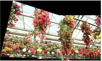
[image:3.595.337.537.210.328.2]Above table shows that as the salt and pepper noise increases after certain value the key points matched are not enough and hence the image stitching is not possible.
[image:3.595.318.565.359.672.2]Figure 3: Resultant Image after stitching images with salt and pepper noise.
Table 3: showing the key points detected and matched with Speckle Noise.
Images Variance Key points Detected Key points Matched
Time Taken
Image 1 Image 2
Set 1 0.1 4312 4403 653 0.0008
0.2 3912 4044 385 0.0006
0.3 3691 3774 267 0.0004
0.4 3521 3654 220 0.0008
0.5 3495 3452 183 0.0002
0.6 3282 3279 124 0.0039
0.7 3113 3072 100 0.0009
0.8 3039 3106 102 0.0008
0.9 2883 2966 103 0.0008
Set 2 0.1 1848 1925 103 0.0176
0.2 1934 1977 55 0.0004
0.3 1908 1830 39 0.0011
0.4 1876 1844 18 0.0009
0.5 1839 1692 23 0.0002
0.6 1770 1601 15 0.0005
0.7 1767 1654 9 0.0007
0.8 1719 1496 15 0.0007
0.9 1627 1501 13 0.0006
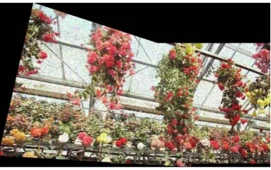
Above table shows that the presence of speckle noise effects the image stitching process to a particular level. Image Stitching is possible even if the noise in the image increases however stitching may not be good enough as compared to images with lower noises.
[image:3.595.61.256.361.483.2]Figure 4: Resultant Image after stitching images with speckle noise.
Table 4: showing the key points detected and matched with Gaussian noise.
Image Mean Key points Detected Key points
Matched Time Taken
Image 1 Image 1
Set 1 Variance=0.5
0.1 2581 2555 26 0.0001
0.2 2541 2719 28 0.0006
0.3 2466 2557 31 0.0011
0.4 2485 2595 29 0.0003
0.5 2507 2556 27 0.0008
0.6 2629 2665 25 0.0006
0.7 2563 2718 27 0.0048
0.8 2732 2735 24 0.0005
0.9 2716 2800 15 0.0008
Set 2 Variance= 0.1
0.1 1936 1850 46 0.0018
0.2 1870 1697 37 0.0004
0.3 1761 1690 34 0.0008
0.4 1882 1676 28 0.0004
0.5 1862 1701 26 0.0012
0.6 1895 1747 17 0.0010
0.7 1963 1892 20 0.0010
0.8 2341 2283 10 0.0003
0.9 2863 3358 13 0.0010
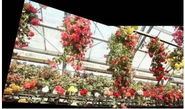
[image:3.595.36.291.517.742.2]Figure 5: Resultant Image after stitching images with Gaussian noise.
Table 5: showing the key points detected and matched with Poisson Noise.
Images Key points Detected Key points
Matched
Time Taken
Image 1 Image 2
Set 1 4766 5233 1211 0.0004
Set 2 1597 1857 343 0.0012
From the above table it is concluded that Poisson noise least affects the image stitching process, as this noise cannot be added externally but from dataset itself.
Figure 6: Resultant Image after stitching images with Poisson noise.
On the basis of above results we get the following comparisons.
[image:4.595.36.282.231.301.2]Figure 7: Graph showing key points matched for set 1 in different noisy images.
Figure 8: Graph showing key points matched for set 2 in different noisy images.
V. CONCLUSION
This paper applies an image stitching algorithm using SIFT as feature detector on images with different types of noises. Each noise is different from another and behaves uniquely. So, the images with different noises are stitched together and a comparison is done based on the results. The key points detected and matched are more in the images when considered without noise but as soon as noise is entered into images the key point detected reduce so does the key points matched. Hence the Image Stitching is affected. From the experimental results we observed that as the amount of noise in the image increases it becomes difficult to stitch the images. On the account of different noises we observe that the key points matched in Gaussian noise are least and highest in the Poisson noise among the noises taken into consideration. Hence it can be concluded that even the presence of small amount of Gaussian noise in image makes it difficult to stitch the images and the Poisson noise least effects the image stitching.
VI. REFERENCES
[1] Image Stitching of Dissimilar Images. Gil Rupert Licu, [2] Seamless Image Stitching Using Structure Deformation
with HoG Matching. Seohyung Lee, Youngtae Park, Daeho Lee. s.l.: IEEE, 2015.
[3] Shape-Preserving Half-Projective Warps for Image Stitching. Che-Han Chang, Yoichi Sato, Yung-Yu Chuang. s.l.: IEEE, 2014.
[4] A survey on image mosaicing techniques. Debabrata Ghosh, Naima Kaabouch. s.l.: Elsevier Inc., 2015.
[5] Efficient Image Stitching of an Image Sequence by Selecting Dominate Frames. Huang, Cheng-Ming and Shu-Wei Lin. 2015.
[6] Analysis of Image Stitching Error Based on Scale Invariant Feature Transform and Random Sample Consensus. Shuang, Dou, et al. s.l.: IEEE, 2015.
[7] Distinctive Image Features from Scale-Invariant Keypoints. Lowe, D. 2004, Vol. 1.
[8] A Comparison of Keypoint Descriptors in the Context of Pedestrian Detection:FREAK vs. SURF vs BRISK. Schaeffer.
[9] Overview of the RANSAC Algorithm. Derpanis, K. G. 2010.
[10]Parallax-tolerant Image Stitching. Liu, F. and Zhang. s.l.: IEEE, 2014.
[image:4.595.63.252.347.458.2] [image:4.595.40.263.502.648.2][13]A Comparative Study of Various Types of Image Noise and Efficient Noise Removal Techniques. Mr. Rohit Verma, Dr. Jahid Ali. 2013. International Journal of Advanced Research in Computer Science and Software Engineering. Vol. 3.
[14]Image De-noising by Various Filters for different Noise.Mr. Pawan Patidar, et al. International Journal of Computer Applications. Vol. 9.