Volume 2, No. 6, Nov-Dec 2011
International Journal of Advanced Research in Computer Science
REVIEW ARTICLE
Available Online at www.ijarcs.info
A Review of Front End and Back End Techniques for ASR
Deepika Sethi *, R. K. Aggarwal
Department of Computer Engineering, National Institute of Technology Kurukshetra – 136119, India
[email protected] [email protected]
Abstract—Speech recognition is an alternative of typing on key-board. It is based on sound-analysis and converts the spelled words into the text. Last few decades have strengthened the foundation of ASR systems. This paper aims to provide an overview of the recognition process. Various feature extraction methods like MFCC, PLPCC etc. are reviewed here. These methods (MFCC and PLPCC) are compared on the basis of their way of processing the speech utterance. Connectionist approach to recognize the speech is explored. Finally experimental results are presented to show that how PLPCC provides more accuracy than MFCC as the number of coefficients increases.
Keywords: ASR, Hidden Markov Models, Mel Frequency Cepstral Coefficients, PLPCC, Time Delay Neural Networks, WER
I. INTRODUCTION
Automatic speech recognition (ASR) is the process of recognizing the word sequence corresponding to the speech signal. Despite the advancements accomplished in the last decades, ASR is still a difficult task because of the increasing size of the dictionary, robustness of the environment and variations in pronunciation.
The traditional method of speech recognition is based on representing the speech signal by its feature vector and using these feature vectors for classification. The two most popular methods of feature extraction are MFCC and PLPCC [1]. To evaluate these feature vectors, HMMs have been successfully applied in ASR as an acoustic model but it suffers from certain drawbacks. Attempts are made to overcome these drawbacks with adoption of ANN (time delay neural network (TDNN) [2] and recurrent neural networks (RNN)) as alternative paradigm for ASR. But ANN failed as a general framework for ASR due to the absence of long term dependencies. In early 1990s, this problem led to the idea of combining HMM and ANN as a single model, named as hybrid HMM/ANN [3].
The organization of the paper is as follows. Section II will provide an overview of ASR system architecture. In the Section III, we discuss the various feature extraction techniques. Section IV presents a number of Connectionists modeling techniques. In section V experimental results are presented and discussed. Finally, the conclusion of the paper will be presented in Section VI.
II. STRUCTUREOFASRSYSTEM
The proposed ASR system architecture comprises of two ends: front end and back end [4] . The front end mainly covers pre-processing and feature extraction. The back end covers acoustic modeling, decision making and language modeling as shown in Fig. 1.
Figure. 1. The architecture of ASR system
A. Preprocessor:
Speech signal is an analog waveform. This kind of the signal cannot be directly processed by the digital systems. Hence, pre-processor performs sampling and quantization to transform the input signal into a form that can be processed by the recognizer [5].
B. Feature Extractor:
The purpose of a feature extractor is to excerpt the required information from the processed signal. The feature extractor discards the irrelevant data while keeping the useful one. The following properties are required for a good feature extractor:
a. Compact features to enable real time analysis. b. Minimum loss of Discriminative information.
C. Classifier:
Once the classes are defined as sequences W of allowable words, a sequence of acoustic feature vectors is selected and a Maximum Posterior criterion is adopted. The classification problem can then be stated as finding the sequence of words W which maximizes the quantity
given by equation 1 [6].
Language Model and is known as the Acoustic Model.
III. FEATUREEXTRACTIONTECHNIQUES
One of the important decisions in any pattern recognition system is the choice of features that can be used and the representation of these features. Speech recognition is such an example. As shown in Fig. 2, the speech signal contains the characteristic information of the speaker (SI) and Environment (EC) in addition to signal message (SM) [7].
Figure. 2. Feature extraction in speech
A Feature Extractor for speech recognition needs to discard maximum of the SI and EC information and allow only the SM information to pass from the speech signal. The ability of FE for speech recognition improves with filtering of SI and EC.
a. SI =⇒Speaker Independence b. EC =⇒Noise Robustness
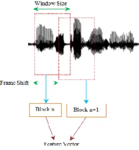
The speech signal is processed in frames with frame size ranging from 15 to 25 milliseconds and an overlap of 50%-70% between consecutive frames as shown in Fig. 3. The overlap between two consecutive frames
Figure. 3. Frame based feature extraction
Is necessary to account for the possibility of a split of an acoustic unit. The feature extraction techniques are broadly classified as temporal analysis and spectral analysis techniques. In temporal analysis, the speech waveform itself is used for analysis, whereas in spectral analysis, spectral representation of speech signal is used. In more than 30 years of recognizer’s research, many different feature extractions of the speech signal have been suggested and tried. The most popular feature representation currently used is the Mel Frequency Cepstral Coefficients (MFCC), another one being Perceptual Linear Prediction Cepstral Coefficients (PLPCC).
A. Mel Frequency Cepstrum Coefficient:
In MFCC, the spectrum is warped according to the Mel Scale, which considers human perception sensitivity with respect to frequencies. The Mel Scale [7] is defined by the equation 2 as follows:
Where f is the frequency in hertz.The speech signal is sent to a high-pass filter given by the equation 3:
(3) Where is the output signal. The value of a usually lies between 0.9 and 1.0. Equation 4 defines the z-transform of the filter [6]:
(4) The goal of pre-emphasis is to compensate the high-frequency part that gets suppressed during the sound production mechanism in humans. The filtered speech signal is segmented into frames of 15~25 ms with optional overlap of 1/3~1/2 of the frame size. Each frame is multiplied with a hamming window in order to keep the continuity of the first and the last points in the frame (to be detailed in the next step). If the signal in a frame is denoted by , then the signal after hamming windowing is , where , the Hamming window is defined by equation the 5:
(5) Different values of α corresponds to different curves for the Hamming window. The signal is transformed from the time domain to frequency domain using Discrete Fourier Transformation (DFT) or Fast Fourier Transformation (FFT), to which the filtering operation can be applied. Fourier analysis is performed through Fourier Transform [8] that for a discrete time signal is given by equation 6:
(6) Where ω is continuous frequency axis
The Fourier transform of is defined by equation 7: (7) The Fourier transform of is given by equation 8:
(8) For the filtering of discrete signal, a number of filters (filter bank) are used. A filter can be defined as a mechanism to pass or suppress energy contained in certain bands. The filter can have different shapes such as triangular, rectangular, Gaussian etc. depending on the requirement [7]. The filter bank output can be written as:
(9)
(10)
B. Perceptual Linear Prediction:
Perceptual Linear Predictive Cepstral Coefficient (PLPCC) [9] is another feature extraction technique, which emulates the human auditory system. There are three main concepts behind PLP. They are (1) critical band frequency selectivity, (2) equal-loudness curve and (3) intensity-loudness power law. The steps involved in the computation of the PLPCC [10] are shown in Fig. 4.
a. Perform frame blocking and windowing on the speech signal.
b. Compute the discrete Fourier transform (DFT) and its squared magnitude.
c. Integrate the power spectrum hence computed within overlapping critical band filter responses.
d. Pre-emphasize the spectrum to simulate the unequal sensitivity of the human ear to different frequencies. e. Compress the spectral amplitudes by taking the cube
root after integration.
f. Perform an inverse discrete Fourier transform (IDFT). g. Perform spectral smoothing on the critical band spectra
using an autoregressive model derived from regression analysis.
h. Use an orthogonal transformation like the KLT or the DCT to compute uncorrelated PLPCC.
i. Optionally filtering can be performed to equalize the variances of the different cepstral co-efficient.
Figure. 4. Computation steps of the PLPCC
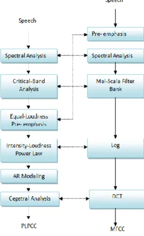
C. Comparison of MFCC and PLPCC:
In this section MFCC and PLPCC are compared on the basis of steps involved in processing the speech signal [11]. MFCC uses the Mel filter banks to model the hair spacing along the basilar membrane of the ear while PLPCC uses the Linear Predictive (LP) analysis and Bark scale to model the auditory like spectrum as shown in Fig. 5. MFCC analysis computes cepstral coefficients from the log Mel-filter bank using a discrete cosine transform. However, in PLPCC analysis, the critical-band spectrum is converted into a small
number of LP coefficients through the application of an inverse DFT to provide autocorrelation coefficients. From the LP coefficients, cepstral coefficients are computed and these form the final static feature vector.
Figure 5. Comparison of MFCC and PLPCC
IV. CONNECTIONISTMODELING
In ASR, many approaches have been used for classification. HMM is a well-known and widely used statistical method of characterizing the spectral properties of the frames of a speech signal. It has been successfully implemented as an acoustic modeler [12]. Although HMM is an effective approach, it suffers from some major limitations. For this reason, in the late 1980’s, many researchers began using artificial neural network (ANN) for ASR but failed to implement it as a general framework for ASR, due to the absence of long term dependencies. In early 1990s this problem led to the idea of combining HMM and ANN as a single model, which was termed as hybrid HMM/ANN.
A. Hidden Markov Model:
The underlying assumption of the HMM is that the speech can be well characterized as a parametric random process and the parameters of the random process can be determined in a precise, well-defined manner. HMMs are the natural extension to the markov chain that produces output observation symbols in any given state. Hence, the observation is a probabilistic function of the state. For a given observation sequence, the state sequence is not observable and therefore hidden. This is why the word hidden is placed before Markov Models. Formally, a Hidden markov model is defined as λ (S, M, A, B, π) [13] where
a. S: Set of states
b. M: Number of distinct observation symbols per states. c. Individual symbols are denoted by
.
e. Each represents the probability of transitioning from state to .
f.
g. B: : Emission Probability or Observation Symbol Probability distribution
h.
i. π : Initial State Distribution: the probability that is a start state.
Given the observation sequence and an HMM model λ = (A, B, π), we compute the probability of O given the model i.e. as shown in Fig. 6.
Figure. 6. Word model for the word “need”
Unfortunately, HMM suffers from some major limitations. One major limitation of conventional HMM is that it does not provide an adequate representation of the temporal structure of speech. Secondly, HMM relies on first order Markov assumption, following which the duration of each stationary segment captured by single state is inadequately modeled. Finally, because of conditional independence assumption, all observation frames are dependent only on the state that generated them, not on the neighboring observation frames, which makes it hard to handle non-stationary strongly correlated frames [14].
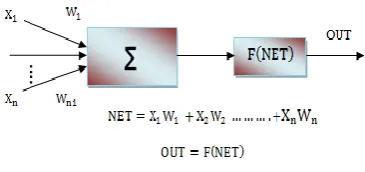
B. Artificial Neural Networks:
The Artificial Neural Network (ANN) is an information processing system, inspired by the working of biological nervous systems, i.e. brain. ANN consists of a large number of highly interconnected processing elements (neurons), work together to solve specific problems as shown in Fig. 7. The various types of ANN have been widely accepted and implemented in numerous areas, especially in speech [15]. To consider the temporal relationships of speech signal, time delay neural network (TDNN) and recurrent neural networks (RNN) have been proposed [2].
Figure. 7. Structure of artificial neuron
TDNN is a neural network approach which addresses both temporal relationship between acoustic events and invariance under translation in time of speech. Superior
speech recognition results can be achieved using TDNN approach. RNN’s provide a very elegant way of dealing with (time) sequential data that embodies correlations between data points that are close in the sequence.The performance of ANN and HMM is compared on the basis of Word Error Rate (WER) [16]. The Word Error Rate (WER) is defined as:
ANN gives considerably better performance than HMM but it has failed due to the lack of long term dependencies.
C. Hybrid HMM/ANN:
The hybrid approach is based on the features of both HMM and ANN. It helped in improving ASR performance significantly [17]. Hybrid HMM/ANN has different architecture, which uses ANN to estimate the state posterior probability for each HMM-state. Bourlard et al. [18] proposed HMM/ANN hybrids for continuous ASR in which a MLP was trained to estimate the posterior probabilities of HMM states, with the ultimate objective of maximizing the posterior probability of a given (left-to-right) Markov model given an acoustic observation sequence . Posterior probabilities can be written as in equation 11.
Where the model is supposed to have states and the acoustic observation sequence
is assumed to be of length. Usually, hybrid HMM/ANN has one state for each phone [19]. In this hybrid HMM/ANN architecture, ANN provides input to the HMM for ASR, as shown in Fig. 8. The training algorithm for hybrid is discriminative at the level of frames and utterance level as well.
Figure 8. Hybrid HMM/ANN for ASR
V. EXPERIMENTALRESULTS
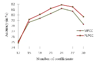
information loss during the process, an overlapping factor of 50% was introduced between adjacent frames. Thereafter, Mel frequency cepstral analysis was applied to extract 12 Mel cepstrum coefficients (MFCC).
Figure. 9. Comparison of MFCC and PLPCC
These coefficients were obtained by applying an inverse DCT (Discrete Cosine Transform) to the log-energy of the filter bank outputs in order to uncorrelate (unassociated/dissociate/unrelated) the parameter (pattern) space. The PLP Cepstral Coefficients
were computed by the standard approach from the Q PLP predictive coefficients. For the final acoustic modeling, original PLP-cepstral representation can be extended with time derivative of PLP Cepstral Coefficients. Fig. 9 shows the results obtained from testing data. The results show that PLPCC provides more accuracy than MFCC as the number of coefficients increases.
VI. CONCLUSION
This paper presents a review of automatic speech recognition system. Firstly, the framework of automatic speech recognition system was presented. The input speech signal can not be directly processed by the recognizer. Preprocessing was carried out to convert it into the form recognizable by the system. To get the feature vectors from the speech signal, various feature extraction techniques were discussed. Connectionist approach used for acoustic modeling has been presented. Finally, experimental results used to compare MFCC and PLPCC were depicted graphically.
VII. REFERENCES
[1]M.A. Anusuya, S.K. Katti, “Front end analysis of speech recognition: a review”, Int J Speech Technol, vol. 14 (2), pp. 99-145, 2011.
[2]A. Waibel, T. Hanazawa, G. Hinton, K. Shikano and K. Lang, “Phoneme recognition using time delay neural networks”, IEEE Trans.Acoust.Speech Signal Process, vol.37, pp. 328-339, March 1989.
[3]H. Bourlard, N. Morgan, “Connectionist Speech Recognition: A Hybrid Approach”, the Kluwer International Series in Engineering and Computer Science, Kluwer Academic Publishers, Boston, Vol. 247, 1994.
[4]Claudio Becchetti and L. P. Ricotti, “Speech Recognition Theory and C++ Implementation”, John Wiley & Sons. [5]J. W. Picone, “Signal Modeling Technique in Speech
Recognition”, Proceedings of the IEEE, Vol. 81 (9), pp. 1215-1247, 1993.
[6]K. Fukunaga, “Statistical Pattern Recognition”, 2nd Edition, Academic Press, San Diego.1990.
[7]Data Driven Feature Extraction and Parameterization for Speech Recognition, M.Tech Thesis submitted to IIT Kanpur, July-2005.
[8]Vrijendra Singh and Narendra Meena, “Engine Fault Diagnosis using DTW, MFCC and FFT”, Proceedings of the First International conference on Intelligent Human Computer Interaction, pp. 83-94, 2009.
[9]H. Hermansky, “Perceptual Linear Predictive (PLP) Analysis for Speech”, J. Acoust. Soc. Am., pp.1738-1752, 1990. [10] H. Hermansky, B. Hanson and H. Wakita, “Perceptually
Based Linear Predictive Analysis of Speech”, Acoustics, Speech, and Signal Processing, IEEE International Conference on ICASSP '85. Vol. 10, pp. 509-512, 1985. [11] Ben Milner, “A Comparison of Front-End
Configurations for Robust Speech Recognition”, IEEE Transaction of Acoustics, Speech and Signal Processing, pp.797-800, 2002.
[12] S. Renals, N. Morgan, H. Bourlard, M. Cohen and H. Franco, “Connectionist Probability Estimators in HMM Speech Recognition”, IEEE Trans. on Speech and Audio Processing, vol. 2 (1), pp. 161-174, 1994.
[13] L.R. Rabiner, “A Tutorial on Hidden Markov Models And Selected Applications In Speech Recognition”, In Proc. IEEE, vol.77, pp. 257–286, 1989.
[14] H. Bourlard, N. Morgan and S. Renals, “Neural nets and hidden Markov models: Review and generalizations”, Speech Communication, Vol. 11, No. 2-3, pp. 83-92,e 1992.
[15] C. Bishop, “Neural Networks for Pattern Recognition”, Clarendon Press, Oxford, 1995.
[16] W.Y. Huang and R.P. Lipmann, “Comparision between Neural Net and Conventional Classifiers”, In Proc. IEEE in Conf. Neural Networks, June 1987.
[17] L. Niles and H. Silverman, “Combining Hidden Markov Models and Neural Network classifiers”, In ICASSP, pp.417– 420, 1990.
[18] H. Bourlard, C. Wellekens, “Links between hidden Markov models and multilayer Perceptrons”, IEEE Transaction of Pattern Analalysis Machine Intelligence, Vol. 12, pp. 1167-1178, 1990.