Volume 3, No. 4, July- August 2012
International Journal of Advanced Research in Computer Science
RESEARCH PAPER
Available Online at www.ijarcs.info
ISSN No. 0976-5697
Histogram Specification with Higher Order Polynomial Functions over R, G and
B Planes for CBIR Using Bins
Dr. H. B. Kekre/Sr. Professor
Department of Computer Engineering, MPSTME. MPSTME, NMIMS University
Mumbai, India [email protected]
Kavita Sonawane/Ph.D Research Scholar Department of Computer Engineering, MPSTME.
MPSTME, NMIMS University Mumbai, India
Abstract: This work Proposes a histogram specification to modify the original histogram such that the intensities form lower level will get shifted to higher side which gives improvement in the results obtained for retrieval of images based on contents. Three polynomial functions proposed in this paper are designed and implemented for modifying the histogram of R, G and B planes of each image. These modified histograms are then partitioned into two parts using the center of gravity. Each partition has got id as ‘0’ and ‘1’. The three planes partitioned into two parts generating the eight combinations from 000 to111, which are used as eight bin addresses. These eight bins are holding the count of pixels having particular range of intensities based on the R, G, and B values falling in specific partition of respective plane’s modified histogram. Bins further are directed to have ‘Total of intensities’ and Average of intensities’ information of the image to be represented as feature vector. Total 21 feature vector databases are prepared by applying the feature extraction process to all 2000 BMP images in the database. Each feature vector in all databases is of dimension 8. This system is tested by comparing 200 query image feature vectors with all feature vector databases by means of the three similarity measures namely Euclidean distance (ED), Absolute distance(AD) and Cosine correlation distance (CD). Performance of the system is evaluated using three parameters PRCP (Precision Recall Cross over Point) Longest String and LSRR (Length of string to retrieve all Relevant images).
Keywords: Histogram Specification, Polynomial function, Bins, Count of Pixels, Total of Intensities, Average of Intensities, ED, AD, CD, PRCP, Longest String, LSRR
I. INTRODUCTION
The core part of any Content Based Image Retrieval system is the approach used to extract the contents of the image and represent them in compact form termed as feature of the image. Image is the high dimensional object consists of thousands of pixels. Feature extraction process reduces the dimension and represents that image and makes the comparison process simple and easy. Important reason behind searching these new techniques for feature extraction is to reduce the feature vector dimension and have good discriminating ability [1][2]. This is one of the important issues we have handled in this work by extracting the entire image content to just eight bins and representing the feature vector of dimension eight. Image contents are broadly classified into two types global and local feature vectors. Global texture features and local features provide different information about the image. It happens because of the variation in the extraction, calculation and representation of the contents. Global features include the descriptors computed on the whole image e.g. contour representations, shape descriptors, and texture descriptors. Local feature includes color shape and texture low level features of the image [3-7].Color represents one of the most commonly used visual features in CBIR systems. Color spaces RGB, Kekre’s LUV, HSV, YCrCb and the hue-min-max-difference are closer to human perception and used widely in CBIR systems.[8-11] Color histogram (CCH) of an image indicates the frequency of occurrence of every color in the image. From a probabilistic point of view, it refers to
Dr. H.B. Kekre et al, International Journal of Advanced Research in Computer Science, 3 (4), July–August, 2012. 330-340
© 2010, IJARCS All Rights Reserved 331 extracted in this system for each database image and
multiple feature vector databases are prepared. When a query image is fired to the system, same set of feature vectors are computed for it. Query and database feature vectors are compared by means of three similarity measures namely Absolute distance (AD), Euclidean distance(ED) and Cosine correlation distance (CD)[18][21-23]. This CBIR system is experimented with database of 2000 BMP images having 20 different classes. Performance of the system for all the approaches used is evaluated using parameters Precision Recall Cross over Point (PRCP), Longest String and LSRR (Length of the String to Retrieve all Relevant)[18], [21].The presentation of the work is organized as follows. Section 2 describes the phases involved in the feature extraction process with implementation details. Section 3
II. HISTOGRAM SPECIFICATION
This technique helps in modifying the image into desired image by transforming the original histogram into new histogram specified by the desired specification function. This is remapping of the original intensities to new scale.
A. Higher order polynomial functions
We have used three higher order polynomial functions as specifications to modify the original histogram before feature extraction. Three polynomial functions proposed and used in this work are given as follows:
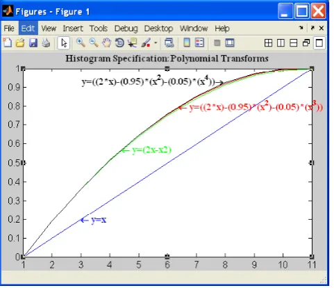
Figure 1. Histogram Specification: Higher Order Polynomial Functions
Equations 1, 2 and 3 are showing the higher order polynomial functions used to modify the histogram. The curves for these three functions are shown in Figure1. We can observe in the Figure1.that when y=x we got straight line and for all other three functions we can see that ‘y > x’, i.e. intensities are being shifted from lower side to higher side. These functions are used to push the histogram more towards the higher intensities so that it will benefit in the feature extraction and to improve the retrieval.
B. Modification of Histogram using Specification
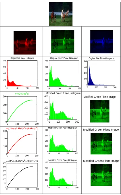
Original histogram intensities can be mapped to new intensities by means of polynomial functions discussed in section 2.1. This mapping and its effect on the image can be seen in the following Figure 2. It shows the image is first separated into three planes R, G and B. Then for each plane histogram is obtained and modified using above three polynomial functions given in eq. 1, 2 and 3.
As shown in Figure 2. Top row shows the Image from Horse class. In second row it is separated into R, G and B planes. In third row original histograms of the three planes are shown below respective plane. Next three rows are
showing the polynomial functions y=
(
2x−x2)
,( ) ( )
( )
( )( )
(
2*x 0.95 * x2 0.05 * x3)
y= − − and
( ) ( )
( )
( )( )
(
2*x 0.95 * x2 0.05 * x4)
y = − − with their
effect on the original histogram shown for blue plane which is reflected in modified histogram images. In these three modified histogram images we found that the intensities are getting shifted towards higher side by means of three polynomials. Green plane images obtained for new histograms are shown beside each modified histogram for each of three polynomials. Same process is applied to other two planes (Red and Blue) histograms.
III. FEATURE EXTRACTION
Efficiency of all the CBIR systems depends on the approach used to extract the image contents and represent them in proper format called feature vector. There are various approaches designed by the researchers from two domains of image processing that are spatial and frequency domain [20][21]. We have used the approach based on histogram specification from spatial domain to extract the feature vectors. The complete feature extraction process is divided in three steps we followed is explained below.
A. CG partitioning
Feature extraction process starts with the separation of image into R, G and B planes. Histogram of each plane is modified using the histogram specification given by equations 1, 2 and 3. After modification the new histograms are partitioned into two parts based on the uniform
distribution of the mass of intensities in two parts. This uniform distribution of mass of intensities is obtained by computing the Center of Gravity. Center of Gravity gives the exact balancing point where two parts of the data will have equal mass. Equation 4 is identifying the formula used to compute the CG. and Figure 3 is highlighting the partitioning of modified blue plane histogram in parts with id ‘0’ and ‘1’. This assignment of id’s to the two parts is applied to each plane.
(
)
∑ = + + + = n i i W n W n L W L W L CG 1 ... 2 2 1 1 (4)(
2)
x x 2
y= − (1)
(
) (
)
( )
(
)
( )
(
2*x 0.95 * x2 0.05 * x3)
y= − − (2)
(
) (
)
( )
(
)
( )
(
2 4)
x * 0.05 x * 0.95 x * 2
y= − − (3)
[image:2.595.54.295.396.603.2]Dr. H.B. Kekre et al, International Journal of Advanced Research in Computer Science, 3 (4), July–August, 2012. 330-340
Where Li is intensity Level and Wi is no of pixels at Li
\
0 100 200 300
0 200 400 600 800
Original Red Image Histogram
0 100 200 300
0 100 200 300 400
Original Green Plane Histogram
0 100 200 300
0 200 400 600 800
Original Blue Plane Histogram
0 100 200 300
0 100 200 300
y=((2*x)-(x2))
0 100 200 300 0
100 200 300 400
Modified Green Plane Histogram
Modified Green Plane Image
0 100 200 300
0 100 200 300
y=((2*x)-((0.95)*(x2))-(0.05)*(x3))
0 100 200 300
0 100 200 300 400
Modified Green Plane Histogram
Modified Green Plane Image
0 100 200 300
0 50 100 150 200 250 300
y=((2*x)-((0.95)*(x2))-(0.05)*(x4))
0 100 200 300
0 100 200 300 400
Modified Green Plane Histogram Modified Green Plane Image
[image:3.595.87.509.62.739.2]Dr. H.B. Kekre et al, International Journal of Advanced Research in Computer Science, 3 (4), July–August, 2012. 330-340
© 2010, IJARCS All Rights Reserved 333
B. Bins formation
Once the id is assigned to each partition of all three planes the next process starts i.e formation of bins. Three
planes, each with two ids gives us 23= 8 combinations
from ‘000’ to ‘111’. Theses combinations are treated as bin addresses to extract the feature vectors.
[image:4.595.86.241.230.356.2]When the feature is being extracted the R, G and B intensities of the pixel of images under process will be taken into consideration. Now, suppose the R value falls in the partition 1of red plane, G in part ‘0’ and B in part ‘1’ then that pixel gets flag ‘101’ assigned to it. This flag itself indicates the pixel’s destination bin address. Same process is applied for each pixel of the entire image and their destination bin addresses will be acquired.
Figure 3. Green Plane Modified histogram with CG Partitioning
C. Feature Vector Generation
Bins formation process lead towards the actual feature extraction. As explained above in section 3.2 the whole process is applied to entire image pixels and their distribution will be shown through these eight bins from 000 to 111. These eight bins are used as feature vector of dimension 8 for comparing the images. Means the size of feature vector based on histogram which is actually of size 256 bins, is reduced to just 8 bins. This greatly reduces the size of feature vector which reduces computational complexity and also the time to compare images. Based on the variation in extraction process we have obtained different types of feature vectors as follows.
• ‘Count of Pixels’:It represents the count of
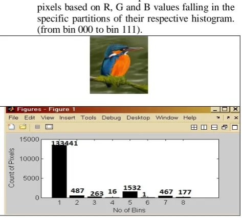
pixels based on R, G and B values falling in the specific partitions of their respective histogram. (from bin 000 to bin 111).
Figure 4. Kingfisher Image with Sample of 8 bins with Count of Pixels
Figure 4 shows the sample kingfisher image with its eight bins from 1 to 8 having the count of pixels. Image size is 128 x128. These 8 bins are showing the distribution of 16384 pixels, we can cross check this by adding the no of pixels counted in all bins, we should get 16384 pixels.
• Total of Intensities: Once the count of pixels is obtained into each bin, R, G and B intensities of these pixels is taken into consideration. We have taken the total of R , G and B intensities falling in each bin separately and it is treated as three new feature vectors in the form of total of intensities ‘Total_R’, ‘Total_G’ and ‘Total_B’ with respective R, G and B color information.
• Average of Intensities: Similar to the ‘Total of intensities’ here we compute the average of R, G and B intensities for the count of pixels in each of the eight bins. This feature vectors are termed as ‘Average_R’, ‘Average_G’ and ‘Average_B’ for R, G and B color respectively.
D. Feature Vector Databases
The feature extraction process explained above in sections from 3.1 to 3.3 is applied to all database images. We have used database of 2000 BMP images having 20 different classes. Based on the types of feature vector with respect to color variation and the computations of contents we have prepared total 21 feature vector databases, each containing 2000 feature vectors of dimension eight. The details of 21 feature databases are as follows:
‘Count of Pixels’- 1 database for each of the three polynomials = (3 databases)
‘Total_R’, ‘Total_G’ and ‘Total_B’ 3 Databases
for each of three polynomial s = ( 9 Databases)
‘Average_R’, ‘Average _G’ and ‘Average_B’ 3
Databases for each of three polynomials = ( 9 Databases)
This way in all we have prepared (3+9+9=21) feature vector databases with each feature vector of dimension 8.
IV. SIMILARITY MEASURE :ED,AD AND CD
In CBIR system’s retrieval of the images is facilitated by comparison process where the query image entered by the user will be compared with the database images. The images are compared by their feature vectors used to represent them. To compare and compute the distance we have used three similarity measure, namely Euclidean distance (ED), Absolute distance (AD) and Cosine Correlation distance (CD) and are given in equations 5, 6 and 7 respectively.
Cosine Correlation Distance
(
) (
)
•
2 ) ( 2 ) (
) ( ) (
n Q n D
n Q n D
Where D(n) and Q(n) are Database and Query feature Vectors resp. (5) Euclidean Distance
[image:4.595.50.287.557.769.2]
Dr. H.B. Kekre et al, International Journal of Advanced Research in Computer Science, 3 (4), July–August, 2012. 330-340
(
)
21
∑
=
− =
n
i
i i
QI FQ FI
D
(6)
)
(
1
I n
I
QI
FQ
FI
D
=
∑
−
(7)
Each of these distance metrics has its own feature and we found all of them are performing better. Euclidean distance varies with variation in the scale of the feature vector but cosine correlation distance is invariant to the scale transformation. Absolute distance also gives better performance for retrieval with less time to compare with reduction in the computational complexity [18].
V. PERFORMANCE EVALUATION OF PROPOSED SYSTEM
Approaches used in this system to extract the features are mainly depending on the histogram specification functions used, bins formation and variations in computing the feature vectors (based on color and statistic). It is essential to determine the role and efficiency of each polynomial and the variation used in feature extraction process. To do this we have used three performance evaluation parameters as Precision Recall Cross over Point (PRCP), Longest String and Length of String to Retrieve all Relevant (LSRR) and are defined as follows[18], [21-25]:
A. PRCP: Precision recall cross over point
The conventional parameter ‘Precision’ gives the measure of accuracy because it concentrates only on the count of relevant images from all retrieved images. Whereas ‘Recall’ keeps track of the count of relevant image from total images of that class in database, in turn we can say it measures the completeness factor. Hence Cross over point of these two parameters termed as PRCP (which varies between 0 to1), is giving the measure of idealness of the CBIR system. PRCP value 0 indicates worst case performance of the system because it states that system could not retrieve the images similar to query. PRCP value 1 indicates the best case performance of the system. It interprets that retrieval result generated for the given query does not contain a single irrelevant image and it has all the images from the database similar to query.
B. Longest String
Whenever query image enters into the system it will be compared with all 2000 images in the database. System calculates the distance between them using the given distance metrics. These 2000 distances will be then sorted in ascending order so that images at minimum distance will appear first in the sequence. But sometimes it happens that very few images will come as initial string of relevant images. If the sorted distances will be travelled further we may found that there is a group of images (more than initial relevant string) which are relevant query are appearing continuously. This possibility cannot be ignored and that is why we have introduced and used this parameter where we can have longest continuous string of images relevant to query.
C. LSRR : Length of String to Retrieve all Relevant
As we have discussed that parameter recall measures the completeness of the system. All CBIR users are expecting that recall should be recall as high as possible.
Now here is the time to check the strength of the system that how long it takes to retrieve all images relevant to query from database. Here we measure the length of traversal required to collect all images relevant to query (to make recall 1) from set of images arranged according the distances sorted in ascending order.
VI. RESULTS AND DISCUSSION
The proposed system’s experimentation is carried in MATLAB with database of 2000 BMP images. We have covered the discussion about the results obtained for each of the 21 feature vector databases. This includes the performance discussion of all small variations in all processes from feature extraction to actual retrieval. It covers the discussion with respect each polynomial, each distance measure, each color and each type of feature vector.
A. Database and Query Image
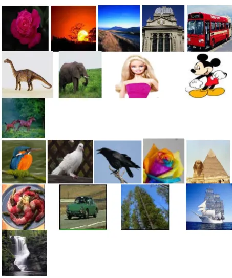
The database used for experimentation is consist of 2000 BMP images having 20 different classes. It includes Flower, Sunset, Mountain, Building, Bus, Dinosaur, Elephant, Barbie, Mickey, Horse, Kingfisher, Dove, Crow, Rainbow rose, Pyramid, Plate, Car, Trees, Ship and waterfall where each class has got 100 images. A sample image from each class is shown in Figure 5.
Ten query images are selected randomly from each class and set of 200 query images is given as query to the system to check its performance with respect to all factors. Results obtained are shown as follows
Figure 5. 20 Sample Images from database of 2000 BMP images from 20 classes
[image:5.595.48.298.46.105.2]B. Results Obtained for PRCP
[image:5.595.314.541.391.663.2]Dr. H.B. Kekre et al, International Journal of Advanced Research in Computer Science, 3 (4), July–August, 2012. 330-340
© 2010, IJARCS All Rights Reserved 335 In Table 2 we found best obtained is ‘6621’ out of
20,000 for poly 3 with CD measure for green color means the precision and recall value is “0.33” . Similarly for count of pixel feature vector we found poly 1 is
giving highest PRCP value as 5556 means precision and recall are at 0.3 for AD measure. Overall observations written below each table are indicating that poly 1 and poly 3 are performing better.
Note: Poly 1 isy=
(
2x−x2)
, Poly 2 is y=(
(2*x) (− 0.95)*( )
x2 −(0.05)*( )
x3)
and Poly 3 is(
) (
)
( )
(
)
( )
(
2*x 0.95 * x2 0.05 * x4)
[image:6.595.142.457.141.232.2]y= − − in entire result and discussion.
Table I. PRCP : TOTAL
SM
R G B
Poly 1 Poly 2 Poly 3 Poly 1 Poly 2 Poly 3 Poly 1 Poly 2 Poly 3
ED 5216 5264 5248 4820 4794 4785 4431 4504 4501
AD 5694 5690 5675 5263 5243 5228 4854 4933 4922
CD 4891 4812 4805 4507 4420 4399 4261 4209 4185
Observation: Poly 1 is better at 6 places out of 9
Table II. PRCP : AVERAGE
SM
R G B
Poly 1 Poly 2 Poly 3 Poly 1 Poly 2 Poly 3 Poly 1 Poly 2 Poly 3
ED 5693 5763 5820 5712 5853 5862 5753 5937 5975
AD 5773 5882 5927 5724 5884 5904 5794 5894 5898
CD 5990 6072 6079 6435 6591 6621 6253 6447 6472
[image:6.595.318.541.498.649.2]Observation: Poly 3 is better at 9 places out of 9
Table III. PRCP : COUNT
SM and Poly Poly 1 Poly 2 Poly 3
ED 5139 5096 5092
AD 5556 5452 5476
CD 5076 5029 5018
Observation: Poly 1 is better at 3 places out of 3
After observing the separate results obtained for three colors R, G and B for feature vector types ‘Total’ and ‘Average’ of intensities; we thought of combining them. To do this we have applied OR operation over the results obtained for R, G and B separately. Results obtained after application of OR criterion over PRCP results of Total and Average of intensities are shown
below in chart 1 and 2 respectively.
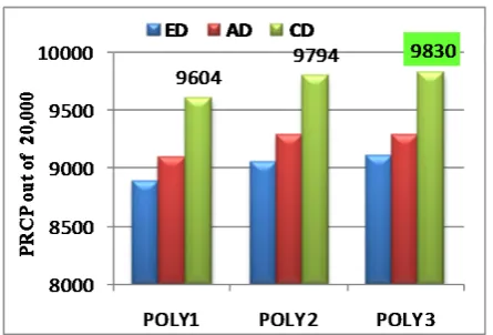
Chart 1. Criterion ‘OR’ for ‘Total of Intensities’
Observation: Chart1 Best result obtained is 7544 for Poly2 with AD measure and
Chart 2. Criterion ‘OR’ for ‘Average of Intensities’
Observation: Chart 2 the best result obtained is for 9830 Poly3 with CD measure.
In above results we observed that the PRCP values are reached to good height after applying the OR criterion. Both charts are highlighting the best results obtained for total and average of intensities. These PRCP values if compared with results obtained before the application of OR criterion, we found very positive difference that precision and recall value for ‘Total of
intensities’ reached to 0.4 from 0.3 and for ‘Average of
[image:6.595.56.277.595.748.2]Dr. H.B. Kekre et al, International Journal of Advanced Research in Computer Science, 3 (4), July–August, 2012. 330-340
[image:7.595.109.489.118.605.2]C. Results for Longest String
Table IV. Maximum Longest String for ‘Count of Pixels’ with ED, AD and CD for Poly 1, 2 and 3
LONGEST STRING FOR COUNT WITH ED AD and CD
Classes
ED AD CD
Poly 1 Poly 2 Poly 3 Poly 1 Poly 2 Poly 3 Poly 1 Poly 2 Poly 3
Flower 11 10 10 13 13 13 12 10 10
Sunset 11 10 12 11 11 10 11 13 11
Mountain 4 4 3 4 3 4 4 4 3
Building 5 4 4 5 4 5 4 4 4
Bus 7 6 7 7 7 8 7 7 7
Diansour 14 19 25 20 27 25 18 19 21
Elephant 4 4 4 4 4 4 4 7 6
Barbie 22 8 8 25 15 17 35 24 25
Mickey 7 11 8 8 11 11 7 6 6
Horses 15 14 17 11 16 15 16 14 14
Kingfisher 4 3 3 4 3 4 3 5 5
Dove 43 43 43 47 47 46 29 28 28
Crow 7 7 7 11 11 11 6 7 6
Rainbowrose 28 27 28 23 27 27 25 24 25
Pyramids 11 10 10 13 12 12 10 10 11
Plates 8 7 7 11 9 9 11 7 11
Car 3 3 3 4 4 3 4 4 3
Trees 8 8 8 7 9 9 10 7 6
Ship 5 5 5 5 5 4 7 6 4
Waterfall 5 4 5 4 5 6 4 4 4
AVG 11.1 10.35 10.85 11.85 12.15 12.15 11.35 10.5 10.5
Observation for Best results Out of 20 Cases in Table 4
ED AD CD
Poly 1 Poly 2 Poly 3 Poly 1 Poly 2 Poly 3 Poly 1 Poly 2 Poly 3
15 9 13 13 12 11 14 9 8
Average of 20 queries is showing that ‘poly 2 is better as compared to other two polynomials
Dr. H.B. Kekre et al, International Journal of Advanced Research in Computer Science, 3 (4), July–August, 2012. 330-340
[image:8.595.144.465.530.752.2]© 2010, IJARCS All Rights Reserved 337 Table V. Maximum Longest String for ‘Total of Intensities’ with ED, AD and CD for Poly 1, 2 and 3
LONGEST STRING FOR TOTAL WITH ED AD and CD
Classes
ED AD CD
Poly 1 Poly 2 Poly 3 Poly 1 Poly 2 Poly 3 Poly 1 Poly 2 Poly 3
Flower 14 12 l 14 15 15 20 21 20
Sunset 16 15 15 22 22 22 22 25 24
Mountain 4 4 3 4 5 4 4 3 3
Building 4 4 5 4 5 5 6 5 5
Bus 16 16 16 17 18 17 10 11 11
Diansour 21 27 25 34 31 30 16 14 15
Elephant 9 6 6 7 6 7 4 4 4
Barbie 13 28 19 7 16 17 8 5 5
Mickey 13 16 15 13 14 14 12 12 12
Horses 17 18 15 20 21 18 19 17 13
Kingfisher 4 4 4 5 6 6 9 7 8
Dove 22 25 25 31 30 32 18 22 22
Crow 18 14 15 21 16 16 8 7 6
Rainbowrose 19 22 20 16 19 20 34 27 28
Pyramids 16 20 20 17 16 14 14 18 18
Plates 5 6 5 5 6 7 7 6 6
Car 4 4 4 4 6 5 4 4 5
Trees 11 11 10 12 11 11 8 8 7
Ship 7 7 5 10 7 7 9 8 8
Waterfall 5 4 6 5 5 5 8 6 6
AVG 11.9 13.15 12.25 13.4 13.75 13.6 12 11.5 11.3
Observation for Best results Out of 20 Cases in Table 5
ED AD CD
Poly 1 Poly 2 Poly 3 Poly 1 Poly 2 Poly 3 Poly 1 Poly 2 Poly 3
10 14 7 7 10 12 14 8 6
Average of 20 queries is showing that ‘poly 2 is better as compared to other two polynomials
Dr. H.B. Kekre et al, International Journal of Advanced Research in Computer Science, 3 (4), July–August, 2012. 330-340
Table VI. Maximum Longest String for ‘Average of Intensities’ with ED, AD and CD for Poly 1, 2 and 3
LONGEST STRING FOR AVERAGE WITH ED AD and CD
Classes
ED AD CD
Poly 1 Poly 2 Poly 3 Poly 1 Poly 2 Poly 3 Poly 1 Poly 2 Poly 3
Flower 9 9 9 15 13 13 20 23 22
Sunset 26 23 24 34 37 37 32 35 36
Mountain 10 9 9 10 9 9 8 9 9
Building 4 5 7 4 5 6 5 5 8
Bus 22 23 22 24 27 25 26 23 25
Diansour 18 27 29 24 28 32 16 22 21
Elephant 8 9 9 10 10 10 10 11 12
Barbie 74 78 78 78 78 80 67 62 62
Mickey 22 21 26 22 20 20 18 12 15
Horses 17 17 16 21 20 19 27 27 26
Kingfisher 11 12 11 10 10 10 13 13 14
Dove 46 45 47 46 42 44 48 46 47
Crow 11 10 11 10 8 9 13 10 9
Rainbowrose 46 44 40 35 34 34 30 30 31
Pyramids 34 26 26 25 22 22 30 29 27
Plates 7 6 6 7 6 9 8 9 8
Car 14 14 14 15 15 15 20 19 17
Trees 11 11 11 9 10 9 12 9 8
Ship 9 10 10 9 9 10 17 18 18
Waterfall 4 5 8 6 5 5 8 9 8
AVG 20.15 20.2 20.65 20.7 20.4 20.9 21.4 21.05 21.15
Observation for Best results Out of 20 Cases in Table 6
ED AD CD
Poly 1 Poly 2 Poly 3 Poly 1 Poly 2 Poly 3 Poly 1 Poly 2 Poly 3
10 9 12 12 6 9 9 7 7
Average of 20 queries is showing that ‘Poly 1’ is better as compared to other two polynomials
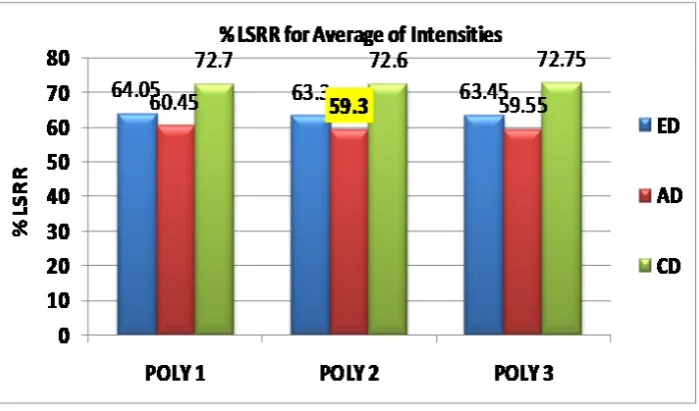
Chart 5. Minimum LSRR for ‘Average of Intensities’ with ED, AD and CD for Poly 1, 2 and 3
Longest string results obtained for ‘Count of Pixels’ are shown in Table IV. Three different colors are showing the discrimination in the results on the basis of three
Dr. H.B. Kekre et al, International Journal of Advanced Research in Computer Science, 3 (4), July–August, 2012. 330-340
© 2010, IJARCS All Rights Reserved 339 the important or noticeable results obtained as average of
20 queries form 20 classes for each polynomial with all three distance measures.
Table V is showing the maximum longest string of relevant images obtained for feature vector ‘Total of intensities’ each of the three polynomials irrespective of the three colors using all three distance metrics. The best value among all three polynomials obtained for each class and each distance measure is highlighted with the respective colors selected for identifying the distance measure separately. Last row gives the average of 20 queries obtained for the 20 results obtained for each polynomial. Important observations made on Table IV are given separately below the Table V.
Table VI shows the results obtained for ‘Average of Intensities’ for three polynomials with three different distance measures. This table highlights the best results obtained for each distance measure separately. ED with green, AD with pink and CD with yellow color. The maximum longest string obtained among results obtained for three polynomials are highlighted with respective color of the distance measure. Last row of the table has average longest string value obtained for 20 queries from 20 classes. When these values are compared we found Poly1 is better as compared to other two polynomials.
D. LSRR
Chart 3, 4 and 5 are showing the results obtained for the parameter LSRR for ‘Count of Pixels’, ‘Total of Intensities’ and ‘Average of Intensities’ respectively. We have computed this parameter for all 200 queries with respect to all the other factors. For ‘Total’ and ‘Average’ feature vector types three results obtained for R, G and B colors separately. We have taken minimum LSRR among the three results of 10 queries from one class and selected as final LSRR for that query class. Charts are showing the average LSRR values of 20 queries (i.e one minimum LSRR from each class) for each polynomial with respect to each similarity measure ED, AD and CD. Charts are highlighting the best results obtained for LSRR with yellow color. According to LSRR definition LSRR should be as low as possible. In above results we can see that minimum percentage of traversal required to collect all relevant images has not crossed 73%. All the resultant LSRR are in range from 59% to 73% in the above results which shows quite good achievement in the results. When we have observed individual results, we found that few queries have got recall value 1 by just traversing the string at 19 to 20% (LSRR).
VII. CONCLUSION
The work explained in this paper is exploring the idea of histogram specification and its use for CBIR. Histogram specification is specified through three new polynomial functions which are shifting the histogram towards higher intensities. The CBIR system explained in this paper is actually based on the bins approach. Bins formation is achieved effectively by partitioning of the histogram using CG i,e center of gravity where CG divides the mass of pixel intensities. After partitioning of the histogram having 256 bins we reduced the size of the feature vector to just 8 bins. This reduces the computational complexity and saves the time for comparing the feature vectors.
Three polynomial functions Poly1 y=
(
2x−x2)
,Poly2 y=
(
(2*x) (− 0.95)*( )
x2 −(0.05)*( )
x3)
andPoly 3 y =
(
(2*x) (− 0.95)*( )
x2 −(0.05)*( )
x4)
are shifting the histogram from lower to higher side each with small shift to right side. All three have given good performance in terms of retrieval. Comparing these results with results obtained for original histogram [12, 13, 16, 17,24], we found that the specification i.e. polynomials used for modifying the histogram are giving better results. Comparing the results on the basis of type of feature vector we found ‘Average of Intensities’ performing better as compared to total of intensities and count of pixels.Comparing the results based on the use of similarity measures ED, AD and CD; we found AD and CD are giving better results as compared to ED.
Performance of the proposed system is evaluated using three parameters PRCP, Longest string and LSRR. PRCP value obtained is 0.5 for ‘average of intensities’ and 0.4 for ‘total of intensities’ shows good achievement in the results as average result of 200 query images.
Maximum longest string obtained among 200 query images is ‘80’ for class Barbie for feature vector average of intensities, 34 for dove class for feature vector ‘Total of intensities’ and 47 for dove class for feature vector count of pixels.
Minimum LSRR obtained among results of 200 queries is just 9% traversal gives 100% recall, this the best results we found for 3-4 queries from class Barbie with feature vector type ‘ average of intensities’.
VIII. REFERENCES
[1] Thomas Deselaers ,“Features for image retrieval”, Ph.D.Thesis, RWTH Aachen University of Technology.
[2] Arnold W.M., Marcel Worring Simone Santini “Content-Based Image Retrieval at the end of the early years”, IEEE Transactions On Pattern Analysis And Machine Intelligence, Vol. 22, No. 12, December 2000.
[3] Sameer Antani, Rangachar Kasturi, Ramesh Jain, “A survey on the use of pattern recognition methods for abstraction, indexing and retrieval of images and video”, 2002 Pattern Recognition Society. Published by Elsevier Science Ltd. Pattern Recognition 35 (2002) 945–965.
[4] Ramadass Sudhir, Lt. Dr. S. Santhosh Baboo “An efficient CBIR technique with YUV Color space and texture features” Computer Engineering and Intelligent Systems, ISSN 2222-1719 (Paper) ISSN 2222-2863, Vol 2, No.6, 2011.
[5] Dimitri A. Lisin, Marwan A. Mattar, “Combining local and global image features for object class recognition”, Intelligente System, Fachbereich Informatik, TUDarmstadt, Germany.
[6] Younes RAOUI, El Houssine, Michel DEVY, “Global and local image descriptors for Content Based Image Retrieval and object recognition”, Applied Mathematical Sciences, Vol. 5, no. 42, 2109 – 2136, 2011.
[7] Sebastian Nowozin, “Object classification using local image features” A report in Computer Vision and Remote Sensing, Technische University¨ at Berlin
[8] P.L. Stanchev, D. Green Jr. and B. Dimitrov, “High level color similarity retrieval,” Int. J. Inf. theories, pp 363–369, April 2004.
Dr. H.B. Kekre et al, International Journal of Advanced Research in Computer Science, 3 (4), July–August, 2012. 330-340
[10] R. Shi, H. Feng, T.-S. Chua and C.-H. Lee, “An adaptive image content representation and segmentation approach to automatic image annotation,” International Conference on Image and Video Retrieval (CIVR), pp. 545–554, 2004.
[11] V. Mezaris, I. Kompatsiaris and M.G. Strintzis, “Ontology approach to object-based image retrieval,” Proceedings of the ICIP, vol. II, pp. 511–514, 2003.
[12] Gi-Hyoung Yoo, Beob Kyun Kim, and Kang Soo You, “Content-Based Image Retrieval using shifted histogram”, ICCS 2007, Part III, LNCS 4489, pp. 894–897, 2007. © Springer-Verlag Berlin Heidelberg 2007.
[13] Shengjiu Wang, “A robust CBIR approach using lLocal color histograms”, Technical Report TR 01-13, October 2001.
[14] Wei-Min Zheng1, Zhe-Ming, “Color Image Retrieval Schemes using index histograms based on various spatial-domain vector quantizes” International Journal of Innovative Computing, Information and Control ICIC International ISSN 1349-4198 Volume 2, Number 6, December 2006.
[15] Sangoh Jeong , “Histogram-based color image retrieval”, psych221/EE362 Project Report, Mar.15, 2001.
[16] H. B. Kekre and Kavita Sonawane, “Bins approach to image retrieval using statistical parameters based on histogram partitioning of R, G, B planes”, International Journal of Advances in Engineering & Technology, Jan 2012.
[17] H. B. Kekre and Kavita Sonawane, “Bin pixel Count, Mean and Total of intensities extracted from partitioned equalized histogram for CBIR”, International Journal of Engineering Science and Technology (IJEST), ISSN : 0975-5462 Vol. 4 No.03 March 2012.
[18] Dr. H. B. Kekre and Kavita Sonawane, “Effect of similarity measures for CBIR using bins approach”, International Journal of Image Processing (IJIP), Volume (6) : Issue (3) : 2012.
[19] H. B. Kekre and Kavita Sonawane, “Feature extraction in bins using global and local thresholding of images for CBIR”, (IJ-CA-ETS) , ISSN: 0974-3596, October ’09 – March ’10, Volume 2, Issue 2.
[20] Yining Deng,B. S. Manjunath, Charles Kenney, “An efficient color representation for image retrieval”, IEEE Transactions on Image Processing, Vol. 10, No. 1, January 2001.
[21] Dr. H. B. Kekre, Kavita Sonawane,“Retrieval of images using DCT and DCT Wavelet over image blocks” (IJACSA) International Journal of Advanced Computer Science and Applications, Vol. 2, No. 10, 2011.
[22] H. B. Kekre, Kavita Sonawane, “Query based image retrieval using Kekre, DCT and Hybrid wavelet transform over 1st and 2nd Moment”, International Journal of Computer Applications (0975 – 8887)Volume 32– No.4, October 2011.
[23] Ajay B. Kurhe, Suhas S. Satonka “Color matching of images by using Minkowski- form distance”,global journal of Computer Science and Technology, Volume 11 Issue 5, version 1.0 April 2011.
[24] H. B. Kekre , Kavita Sonawane, Bins formation using CG based partitioning of histogram modified using proposed polynomial transform ‘Y=2X-X2’for CBIR,
[25] Julia Vogela, Bernt Schiele, “Performance evaluation and optimization for Content-Based Image Retrieval” Journal of the pattern recognition society www.elsevier.com
Dr. H. B. Kekre has received B.E. (Hons.) in Telecomm. Engg. from Jabalpur University in 1958,M.Tech (Industrial Electronics) from IIT Bombay in 1960, M.S. Engg. (Electrical Engg.) from University of Ottawa in 1965 and Ph.D. (System Identification) from IIT Bombay in 1970. He has worked Over 35 years as Faculty of Electrical Engineering and then HOD Computer Science and Engg. at IIT Bombay. For last 13 years worked as a Professor in Department of Computer Engg. at Thadomal Shahani Engineering College, Mumbai. He is currently Senior Professor working with Mukesh Patel School of Technology Management and Engineering, SVKM’s NMIMS University, Vile Parle(w), Mumbai, INDIA. He has guided 17 Ph.D.s, 150 M.E./M.Tech Projects and several B.E./B.Tech Projects. His areas of interest are Digital Signal processing, Image Processing and Computer Networks. He has more than 450 papers in National / International Conferences / Journals to his credit. Recently twelve students working under his guidance have received best paper awards. Five of his students have been awarded Ph. D. of NMIMS University. Currently he is guiding eight Ph.D. students. He is member of ISTE and IETE.