R E S E A R C H
Open Access
An initial analysis of packet
function-aware extension to Dijkstra algorithm for
wireless networks
Mustafa Arisoylu
Abstract
In this paper, we promote the packet function (e.g., packet size) -aware extension of the Dijkstra algorithm (i.e., PFA_SPF) as a base algorithm where any routing protocol can evolve it and integrate it with appropriate routing metrics. In particular, we propose a generic algorithm for packet function-aware path setup for multi-hop networks. The algorithm is based on a generic and novel extension of the classical Dijkstra algorithm in which the cost of each link is a non-negative-valued function of packet parameter(s) (e.g., packet size) rather than a scalar value. The algorithm minimizes the sum of the cost functions (e.g., total transmission delay or total energy consumption) experienced by each packet (e.g., maximizing the throughput) from the source to the destination node. We did initial analysis based on simulation of the algorithm for various random multi-hop wireless networks (e.g., 802.11), utilizing realistic link delay models. Finally, we demonstrate the initial significant potential performance improvements of our algorithm over the existing prior art.
Keywords: Path setup, Wireless networks, Packet function aware
1 Introduction
Multi-hop wireless and wired networks and associated protocols are widely used and studied for various applica-tions for residential, military, and emergency networking [1–74].
1.1 Wireless network types
Depending on the deployment scenario, wireless net-works can be mobile or static. Accordingly, these netnet-works can exhibit a wide range of characteristics in terms of connectivity, delay, bandwidth, and topology over time.
On one hand, static multi-hop wireless mesh net-works got significant attention due to various commercial deployments such as residential multi-hop wireless net-works (e.g., among residents or within a resident) or community wireless networks [14, 46, 50–52]. In this case, mostly the network nodes/user equipment are static or minimally mobile.
Correspondence: [email protected]
Ericsson Inc R&D Silicon Valley, 250 Holger Way, 95134 San Jose, CA, USA
On the other extreme, some wireless networks may not have continuous network connectivity due to the mobility and/or extreme conditions of the environment so that even the well-known ad hoc routing proto-cols such as AODV [75] and DSR [76] do not work well. Such networks in the literature are called delay-tolerant networks [53–57]. These networks range from terrestrial mobile networks and military ad hoc net-works to deep space communications. The overall rout-ing/path setup is based on store-and-forward routing so that the data is incrementally stored and forwarded over the network until it eventually reaches the intended destination.
Even though the results of this paper apply both static and mobile networks (including the delay-tolerant net-works), the basic network model used in this paper is from an experimental static wireless network deployment and the simulations in this paper are based on this net-work model. Therefore, the initial focus and motivation of the findings of this paper is towards static wireless networks.
1.2 Packet size distributions
Applications, such as File Download, VoIP, and Video on Demand, generate diverse packet sizes [1–7]. For instance, a file download application mostly utilizes the maximum transmission unit (MTU) (e.g., 1500 bytes), to maximize the throughput, whereas Voice over IP (VoIP) applications generate smaller packets of about 200 bytes in size to min-imize the delay. In other words, it is observed that there is diversity in the packet size distribution over the Inter-net, and the amount of traffic with small packet sizes is significant.
1.3 Wireless MAC layer challenges and solutions
There is a vast number of MAC layer wireless proto-cols designed for specific applications differing from each other in various aspects. However, in almost all the cases, there is a MAC layer overhead time per packet trans-mission resulting from various protocol implementation details. As an example, 802.11 inherits such MAC layer overhead time as shown in [16, 19, 21].
802.11 with multiple data transmission rates is known to assign a fair chance to each link to access the channel. Therefore, the throughput achieved on each contending link, regardless of its data transmission rate, may end up being the same low rate (i.e., max-min fair rate), which is even lower than that of the slowest contending link in the network. This effect, which is generally called the harmonic mean effect of 802.11, significantly reduces the overall network throughput. Various research papers studied this anomaly of 802.11 and other interference-limited multi-hop networks, as in [14, 16–20, 25].
Liu et al. [17] and Korakis et al. [18] propose and imple-ment a novel cooperative MAC layer mechanism attempt-ing to solve the 802.11 throughput problem mentioned earlier.
Dunn et al. [19] propose to set the MTU value of an 802.11 link based on the corresponding data transmission rate to increase the overall throughput while providing a proportional-like fairness rather than max-min type fairness among the contending links in the network.
In [22], VoIP packets are aggregated to minimize the MAC layer overhead of the system while still meeting the delay requirements.
Channel assignment in multi-channel wireless networks (e.g., 802.11/WiFi) is also an active area of research where multiple algorithms are devised to assign optimal chan-nels to each link [32–34] in order to reduce the interfer-ence within the network.
1.4 Coding techniques and transport layer efforts There is also research on multi-path routing in wireless networks [8] utilizing coding techniques such as digital
fountain codes [9, 10]. Given that a message withkpackets is encoded into n packets for transmission, the digital fountain code allows the receiver to recover the orig-inal k packets as long as any k out of n packets are received. In such a setup, receiving the packets in order is not a requirement/limitation anymore such that as long as the receiver receives enough number of packets regardless of the order, the original message can be recovered.
Other coding techniques with multicasting is also dis-cussed in various novel research papers [58, 59] where authors designed CodePipe via opportunistic routing and random linear network coding (along with intra- and inter-batch coding) which not only leads to simple coor-dination among nodes but also increases the multicast throughput.
In addition to the above multi-path and coding tech-niques, as a transport protocol, TCP-friendly rate control for wired and wireless networks is also studied in vari-ous papers [11–13], so that the adverse effects of wireless packet losses and out-of-order packet delivery to TCP can be avoided while still avoiding the congestion collapse in the network. In fact, both the coding techniques as well as TCP-friendly transport layer solutions above can be inte-grated for an end-to-end reliable and TCP-friendly rate control.
2 Related work
In this section, we provide an overview on the related work covering MAC and routing layer solutions for wire-less mesh networking.
2.1 Routing metrics and protocols
Depending on the optimization objective of the path setup algorithm, and the related MAC layer protocol character-istics, the link cost metrics can be a function of the packet characteristics, link transmission rates, hop count, link packet loss rates, and MAC layer overhead parameters rather than fixed scalar values. In [46], a set of route met-rics are compared in static as well as mobile network sce-narios, namely, hop count, per-hop round trip time [47], expected transmission count [44], and per-hop packet pair delay [48].
One of the basic metrics being used in wired as well as wireless networks is the hop count. However, it does not take into account any delay, bandwidth, and packet loss rate and characteristics and may end up with non-optimal paths.
direction of a wireless link and computes the delivery ratio (over a sliding window) to calculate the expected trans-mission count (i.e., ETX= 1/(delivery ratio_f×delivery ratio_r) where the delivery ratio_ f/r refers each direc-tion of the wireless link. In this method, the probe packet sizes are fixed and not representing the real traffic packet size mix and they are mostly transmitted at the network basic rate. Therefore, in the ETX model, the packet size as well as the different transmission rates are not included in the model.
On the other hand, ETT improves ETX via taking into account the differences in link transmission rates such as ETT = ETX × S/B where S is the packet size of the probe chosen and B is the estimated bandwidth of the link. Another improvement of ETT over ETX is that ETX would prefer a heavily congested link (which has lower loss rates) over a lightly congested link (which has a higher loss rate). Introducing the throughput met-ric into its cost calculation, ETT aims to address this issue.
However, ETT still uses fixed size of the probe (for data packets) and specifies the cost metric accordingly and does not mention any packet function (or packet size) -dependent path setup.
A medium time metric (MTM)-based method, which is studied in [23, 24], minimizes the end-to-end transmis-sion delay of a packet. The model to calculate the metric is similar to the previous ones such that T =(overhead
+ S/B)/rel where overhead is the per packet overhead of the link and S is the size of the packet and B is the bandwidth of the link. Finally, rel is the reliability index which is the same as the delivery ratio of the packets. In that respect, one can see that MTM= ETX× over-head+ETT. The proposal in the end is to optimize the path setup for 1500-byte packet size only and for some additional reliability metrics. Even though this study took into consideration the packet size, in the end, they have end up optimizing the path setup for 1500-byte packets. However, our initial analysis as well as findings in this paper suggests that indeed packet size is an important parameter to be considered to optimize the path setup. Please note that packet size is just a sample parameter for our algorithm; indeed, it can be any packet function that the network operator may choose to optimize for path setup.
In this paper, we simulated both hop count as well as link metric for 1500 bytes (with respect to our network model which is in alignment with MTM [23]) in comparison to our proposed metric (e.g., packet function/size) over Dijkstra as well as extended version of Dijkstra algorithm. As known, many link state routing protocols for wired and wireless networks (e.g., OLSR [29], OSPF [28, 31], IS-IS [30], MCLSR (multi-channel link state routing) [15], CEDAR (a core-extraction distributed ad hoc routing
algorithm) [35], TILSRP (trust integrated link state rout-ing protocol for wireless sensor networks) [36]) are takrout-ing Dijkstra algorithm as a base and build the protocol on top of it.
Accordingly, various routing metrics are used by these routing protocols. For instance, MR-LQSR (multi-radio link-quality source routing—utilizing ETT/WCETT weighted cumulative expected transmission time metric) [49] is another link-state routing protocol. In MR-LQSR [49], expected transmission time (ETT) of a packet over the link is a function of the loss rate and bandwidth of the link. The authors consider the combination of the MTM [23] and the expected transmission count metric (ETX) [44] as the expected transmission time metric (ETT) and furthermore added a weighted factor for channel diver-sity which is referred as weighted cumulative expected transmission time metric (WCETT).
2.2 Cooperative communications
The fundamentals of the cooperative communications assume a network model with three nodes A, B, and C. A and C have a low throughput link whereas A and B as well as B and C have high throughput links. The coop-erative communications suggests using the multi-hop higher throughput links wherever appropriate [37–43]. In a sense, our method proposes an extended idea where the cooperative communications are performed based on a packet function (e.g., packet size) in an optimal way.
As mentioned before, Liu et al. [17] and Korakis et al. [18] propose and implement a novel cooperative MAC layer mechanism to increase the performance of the IEEE 802.11 MAC protocol. In this new proposed MAC, they allow an intermediate helper node to act as a relay when-ever it is appropriate. Howwhen-ever, the network model they use to decide to use the relay node or not does ignore the MAC layer overhead.
2.3 Packet size-aware path setup
In [21], the authors conducted experiments to measure the transmission delay experienced by packets with differ-ent sizes. Based on these measuremdiffer-ents, the transmission delay on an 802.11 link is modeled as a function of the MAC overhead time, packet size, and the effective trans-mission rate, as in [19] and in alignment with [23, 24].
Next, in [21], a simple packet size-aware path selection mechanism is implemented as a Linux kernel module uti-lizing the netfilter framework for a small network, and the corresponding performance is evaluated through various experiments.
However in [21], the authors do not provide any generic solution for the packet size-aware path setup.
2.4 Our contribution
In this paper, we have extended the classical Dijkstra algo-rithm considering the link costs/metrics are functions of packet and link parameters (e.g., packet size, link rate) to minimize the total cost function (e.g., transmission delay, energy consumption). The algorithm proposed in this paper is a generic algorithm which works for any network (e.g., wired or wireless) as long as the cost func-tions of the links are non-negative valued. In this paper, we not only devise such an algorithm but also simulate the algorithm for packet size-aware path setup over a basic 802.11-based multi-hop wireless network model as an initial example and demonstrate the significant poten-tial performance improvements of our algorithm over the existing prior art (i.e., minimum hop-based path selection and path optimized for 1500 bytes).
The aim of this paper is to present an interesting and novel idea extending the classical path setup algorithms and trigger additional investigation on this subject. In other words, in this paper, we are not proposing a com-plete routing protocol; instead, we are showing the poten-tial of a packet function-aware path setup algorithm as an extension to Dijkstra over a basic fundamental net-work model. Our proposal in this paper is to promote the packet function-aware extension of the Dijkstra algorithm as a base algorithm where any appropriate routing proto-col can evolve and integrate it (with other routing metrics discussed above) and build on top of it. Therefore, in this paper, it does not make sense to compare our extension to Dijkstra Algorithm to full-fledged routing protocols. As a future work, we are considering to build a routing protocol based on the PFA_SPF and compare it with the existing routing protocols through simulations as well as experiments over real deployments.
It is important to note that the sole focus of this paper is the network layer performance optimization. The per-formance interactions with higher layer protocols (e.g., transport layer protocols TCP, UDP, or application layer protocols) are outside the scope of this paper and left as a future work. Especially, TCP performance may be adversely affected by out-of-order packet delivery since our method can generate multiple paths for a single TCP connection.
In addition to that as mentioned in the previous section, there are various research on TCP-friendly rate control
techniques along with multi-path and digital fountain type codes (for applications from file downloads to Voice and Video). This overall networking solution does not require in-order delivery of packets to the receiver. Therefore, as an example, the PFA_SPF algorithm can easily be utilized in such network models.
The rest of the paper is organized as follows: Section 3 presents the proposed algorithm. Section 4 discusses a sample network model. Section 5 presents the simula-tion results of the proposed algorithm where the packet parameter is the packet size and the objective is to min-imize the total transmission delay over various randomly generated networks. Section 6 concludes the paper and mentions the potential future work.
3 The packet function-aware shortest-path first (PFA_SPF) algorithm
In this section, we propose an algorithm that finds the shortest path between a source node and all the other nodes in the network for all possible values of the related packet parameter (e.g., packet size).
The algorithm is a novel extension of the Dijkstra’s algorithm (see [26] and [27]) that originally assumes scalar link costs. However, our algorithm assumes the cost of each link to be a non-negative-valued function of some packet parameter such as packet size. We call our algorithm “packet function-aware shortest-path first algorithm” (PFA_SPF).
The algorithm solves any shortest-path computation problem in which the link costs are non-negative-valued functions of a packet attribute or some other network-related attribute rather than scalars. Any routing proto-col based on our extended version of Dijkstra algorithm (PFA_SPF) can decide on the cost metrics (e.g., it could be packet size-based delay or energy consumption) and add other dimensions to the cost (e.g., loss rate, channel state) and use an evolved version of the algorithm to be able to realize a dynamic and optimized path setup.
In the original Dijkstra algorithm, a shortest-path tree is constructed from a source node to all the other nodes in the network. The PFA_SPF algorithm presented in this study possibly generates multiple shortest-path trees that are associated to a packet parameter (e.g., packet size) range. The shortest-path trees as well as the related packet parameter ranges are computed in the PFA_SPF algorithm.
LetGbe the graph composed of a set of nodesV and a set of linksLconnecting the nodes. Let nodeS∈Vbe the node from which the shortest-path trees to all other nodes in the network are computed.
LetP(x) be the set ofpermanently labeled nodes as a function ofx. Please note that the domain of the func-tionP(x)is an interval on the real line (e.g., [0, 1500)bytes whenxrepresents packet size), whereas the range of the function is set of set of nodes. As an example:
P(x)=
⎧ ⎪ ⎪ ⎨ ⎪ ⎪ ⎩
A= {a1,a2,. . .,an}, forxa≤x<xb B= {b1,b2,. . .,bn}, forxb≤x<xc
· · · ·
Z= {z1,z2,. . .,zn}, forxy≤x<xz
where the set of nodesA,B,. . .,Zdo not have to be mutu-ally exclusive; that is, any two sets can share a node (for instance,a1can be equal tob2).
The function P(x) has a property such that if P(I(xa,xb)) = B, then P(I(x1,x2)) = B for every
I(x1,x2) ⊂ I(xa,xb). Conversely, ifP(I(xa,xb)) = Aand P(I(xb,xc))=A, then
P(I(xa,xb)∪I(xb,xc))=P(I(xa,xc))=A.
LetDj(x) be the distance from node jto node S as a function ofx. LetD(x)be the vector of distances from all the nodes in setV to the nodeS as a function ofx; i.e.,
D(x)=[. . .,Di(x),. . .] fori∈V.
Letdi,j(x)be the cost of link(i,j)∈Las a function ofx.
Letd(x)be the array of link costs as a function ofxfor all the links inLin the network; i.e.,d(x) =[. . .,di,j(x),. . .]
fori,j∈V.
LetNHj(x)be the next-hop node for nodejas a function ofx. LetNH (x)be the vector of next-hop nodes for all the nodes as a function ofx. Basically, the vector of such next-hop nodes specifies the spanning trees from nodeSto all other nodes in the network as a function ofx.
When the domain of any of the above functions, sayf(x), is restricted toI(xa,xb), it is denoted asf(I(xa,xb)). For instance, the functionP(x)for any interval such asxa ≤ x<xbis denoted asP(I(xa,xb)).
Let minF{f1(x),f2(x),. . .,fn(x)}be the minimum
func-tion of funcfunc-tionsf1(x),f2(x),. . .,fn(x). As an example, if
f1(x)=xandf2(x)=4 for 0≤x<∞, then
minF{f1(x),f2(x)} =
x, for 0≤x≤4, 4, forx>4.
The PFA_SPF algorithm can be described as one initial-ization stage and two functions recursively calling each other.
The detailed description of the algorithm is as follows.
3.1 Detailed description of the algorithm
Initialization:
• Let the largest interval beI(x0,xm). • P(I(x0,xm))= {S}
• Di(I(x0,xm))=
di,s(I(x0,xm)), for alli∈N(S) ∞, for alli∈/N(S)
• NHi(I(x0,xm))=
{S}, for alli∈N(S)
∅, for alli∈/N(S) whereN(S)is the set of neighbor nodes ofS.
• Callfind_minimum_distancefunction with
parameters:
P(I(x0,xm)),I(x0,xm),NH (I(x0,xm)),D(I(x0,xm)).
find_minimum_distancefunction with parameters:
P(I(xa,xb)),I(xa,xb),NH (I(xa,xb)),D(I(xa,xb))
• Find the node(s) that has the minimum distance to nodeS for the intervalI(xa,xb):
minFj∈/P(I(xa,xb)){. . .,Dj(I(xa,xb)),. . .}
=
⎧ ⎪ ⎪ ⎨ ⎪ ⎪ ⎩
Di1(x), forx∈I(xa,x1)
Di2(x), forx∈I(x1,x2)
· · · ·
Din(x), forx∈I(xn−1,xb)
where{i1,i2, . . . ,in}are the nodes that have the minimum distance to nodeS in intervals[xa,x1),
[x1,x2),. . .,[xn−1,xb), respectively. • Letx0=xaandxn=xb.
• Fork=1ton
– Add the minimum distance nodes to the permanently labeled sets:
P(I(xk−1,xk))=P(I(xa,xb))∪ {ik}
– If the permanently labeled set consists of all the nodes in the network, then exit the function; i.e., ifP(I(xa,xb))=V, thenexit the function.
– Update the next-hop entries for new intervals for all the nodesh∈Vin the network:
NHh(I(xk−1,xk))=NHh(I(xa,xb))
– Callupdate_nexthop_distancesfunction with parameters:P(I(xk−1,xk)),I(xk−1,xk),
NH(I(xk−1,xk)),D(I(xk−1,xk)),ik.
update_nexthop_distancesfunction with parameters:
• Update all the distances to the source node for the nodes that are not in the permanently labeled set: For all node(s)j∈/P(I(xa,xb)),
Dj(I(xa,xb))
=minFdi,j(I(xa,xb))+Di(I(xa,xb)),Dj(I(xa,xb))
=
di,j(x)+Di(x),xp0 ≤x<xp1. . .xpm−1 ≤x<xpm
Dj(x),xq0 ≤x<xq1. . .xqn−1 ≤x<xqn
Here, the pointsp0,. . .,pm,q0,. . .,qndefine a partitioning of the intervalI(xa,xb)such that for each pi, there exists aqj, except for some which are equal to the end pointsxaandxb. Let
Yj= {y0=xa,y1,. . .,yn+m+1=xb}be the ordered set of these points for nodej.
• Update the next-hop node entries: NHj(x)
=
i, xp0 ≤x<xp1. . .xpm−1 ≤x<xpm
NHj(I(xa,xb)),xq0 ≤x<xq1. . .xqn−1 ≤x<xqn • LetY= ∪jYj= {y0=xa,y1,. . .,yk−1,yk=xb}be
the ordered set all partition points for all nodes j∈/P(I(xa,xb)).
• Forr=1tok, find the minimum distance for each sub-interval by callingfind_minimum_distance with parameters:
P(I(yr−1,yr)),I(yr−1,yr),NH (I(yr−1,yr)),
D(I(yr−1,yr)).
As can be seen, the proposed algorithm implements a recursive method in which thefind_minimum_distance
function calls the update_nexthop_distancesfunction and vice versa. The stopping criterion for the algorithm is P(I(xa,xb)) = V in the find_minimum_distance function; i.e., the algorithm stops when the permanently labeled set for the intervalI(xa,xb)spans to the entire set of nodes in the network.
The complexity of the original Dijkstra algorithm is O(|V|2) in the worst case (see [27]). In comparison to the Dijkstra algorithm, the complexity of the PFA_SPF algorithm isO(|I| × |V|2) in the worst case where|I|is the maximum number of identified subintervals, such as packet size-based subintervals in case of packet size-aware cost functions. Note that this is the worst case complexity since the PFA_SPF algorithm finds the common shortest-path tree until the next subinterval is identified. Then, the algorithm adds the new shortest-path tree for the new subintervals and continues until the next subinterval leads to a new tree or the stop condition of the algorithm is met. In other words, the algorithm may find different number of subintervals for each node separately, so|I|being the maximum is a worst case bound. However, intuitively, the
average number of subintervals over the nodes would give a better estimation on the complexity.
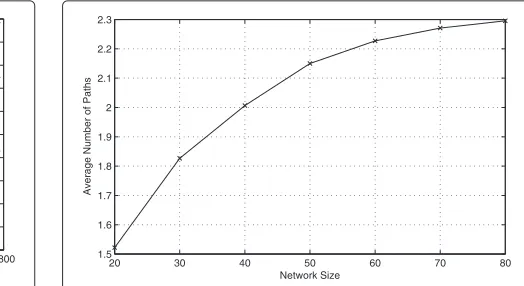
The value of |I| depends not only on the topology of the network including the number of nodes|V|and the number of links |L|but also on the link cost functions. However, to have an idea on the complexity of the algo-rithm through empirical data obtained via our simulations over 4000 random network topologies, one can refer to Fig. 10 which shows the average number of paths vs. net-work size. As can be seen in the figure, the average number of paths or the average number of subintervals is from 1.5 to 2.3 over 4000 random networks of 20 to 80 nodes. This clearly indicates that the complexity of the PFA_SPF algo-rithm is at most 2.3 times that of the Dijkstra algoalgo-rithm for ensemble of 4000 random networks.
The explicit formulation of the upper bounds to the worst case complexity of the algorithm with respect to the link cost function types, the number of nodes(|V|), and links(|L|)is left as a future work.
Notice that the PFA_SPF algorithm is optimal since it is equivalent to the Dijkstra algorithm by construction. One way to prove this is to fix the value of the packet parameter in question (e.g., packet size) in the PFA_SPF algorithm to obtain the Dijkstra algorithm optimized for that packet parameter value. The PFA_SPF algorithm can be seen as a generalization of the Dijkstra algorithm for arbitrary link cost functions.
In the next section, we simulate the PFA_SPF algorithm over randomly generated networks.
4 Sample network model
In this paper, as a sample network model, we utilize the network model in [19, 21] (in alignment with [16, 24]), which is based on experimentation and analysis of multi-hop 802.11 network deployments where all the nodes in the network are in the same contention neighborhood. Note that our algorithm is not limited to this network model; the reason to choose this network model is to present the potential benefits of our algorithm over a basic and fundamental setup.
In addition to that, in real-life deployments, there are various scenarios (as discussed in the “Introduction” section) where a larger network is divided into relatively smaller number of nodes on a single channel where the links of the same channel can stay in the same contention neighborhood.
4.1 Delay and throughput model
As in [19, 21], the transmission delay of a packet over link iwith sizePis modeled approximately as
di(P)=(θi+P/bi) (1)
Please note that the MTM of [24] that is discussed in the earlier sections (i.e., T = (overhead + S/B)/rel) is very similar to the model above where only variable rel (i.e., reliability or the delivery ratio) is not explicitly rep-resented in the model above. However, since 1/rel is a coefficient, through measurements, it is represented by the overall model through measurements.
The throughputTi(P)of a flow on a single 802.11 link is assumed as follows:
Ti(P)=P/di(P) (2)
Considering the harmonic mean effect of 802.11 (in other words, the long-term fair-channel access behavior of the contending 802.11 wireless links), the throughput of a flow traversing multiple 802.11 links is assumed as
R= P
i
di(P) = P
i (θi+
P/bi) (3)
Equations (1), (2), and (3) assume that packet sizes are equal toP.
Please note that Eq. (3) is validated in [21] through real 802.11 multi-hop experimentation for up to four nodes. In this paper, we use this model over simulations with increased network size. As our proposed PFA_SPF algo-rithm is not specific to 802.11 or any other MAC layer protocol, we believe that using Eq. (3) above for increased network sizes in our simulations in this paper is sufficient to present not only the functionality but also the potential benefits of our algorithm. As mentioned previously, our aim in this paper is to present an interesting and novel idea extending the classical path setup algorithms and trigger additional investigation on this subject.
4.2 Validation of the model
To validate this model, in [21], the authors performed var-ious experiments to estimate parameters such as the over-head timeθiand effective bit ratebifor each transmission rate.
Based on the estimations in [21], the delays,dx(in mil-liseconds), to send a packet with sizeP(in bytes) for an 802.11 link with transmission rates 1, 2, 5.5, and 11 Mbps are as follows
d1 Mbps=1.69+0.0094×P
d2 Mbps=1.26+0.0047×P
d5.5 Mbps=1.04+0.0016×P
d11 Mbps=1.06+0.0008×P
(4)
In [21], multi-hop path performance measurements to validate the above model are conducted and verified. The transport protocol that was used in the experiments for devising the above network model was UDP (with infinite demand) over single and multi-hop paths. The size of the packets belonging to this traffic is kept constant through-out each experiment. However, TCP-based experiments
for validation of the model along with the benefits have been conducted as well (see [21] for details).
5 Simulation results
In this section, we present the analyzed scenarios as well as the simulation results of the proposed path setup algo-rithm over various network topologies for the random networks defined in Section 4. We have used the sample network model of this paper that we have obtained via real deployment setup experimentations and extended it via simulations. The link cost metrics are chosen to be the transmission delay as a function of the packet size as well as effective bit rate and overhead time as defined in Section 4. In these simulations, we compute the PFA_SPF algorithm and find possibly multiple shortest-path trees from the source node to all other nodes in the network where each tree is optimized for an optimum packet size interval. Based on these packet size intervals, we compute the throughput gain of the algorithm based on our sample network model with respect to the minimum hop count metric as well as the method optimized just for 1500 bytes. The simulations presented in this paper is developed using Python programming language.
5.1 A sample network
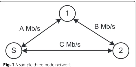
In this example, we trace the PFA_SPF algorithm step by step for a sample three-node network. We consider the topology in Fig. 1 with three links with ratesA = B = 5.5 Mbps andC=2 Mbps.
From (4), the transmission delays for the 2-Mbps and 5.5-Mbps links are as follows:
d2 Mbps=1.26+0.0047x=dS,2(I(0, 1500))
d5.5 Mbps=1.04+0.0016x=dS,1(I(0, 1500)) =d1,2(I(0, 1500))
wherexis the packet size in bytes. As noted before, the transmission delay of a link is considered to be the link cost.
The steps of the PFA_SPF algorithm can be traced for this network as follows:
Initialization:
• Assuming MTU is 1500 bytes, the overall interval is I(0, 1500).
• P(I(0, 1500))= {S}
• D1(x)=dS,1(x)=1.04+0.0016x, forI(0, 1500)
D2(x)=dS,2(x)=1.26+0.0047x, forI(0, 1500) • NH1(x)=NH2(x)= {S}, forI(0, 1500).
• Call functionfind_minimum_distancewith parameters:
{S}, [ 0, 1500), [{S},{S}] ,
[(1.04+0.0016x),(1.26+0.0047x)]
find_minimum_distance:
• Find the nodes that have minimum distance to node S forI(0, 1500):
minFj∈/P(I(0,1500)){D1(I(0, 1500)),D2(I(0, 1500))} =
D1(I(0, 1500))
• P(I(0, 1500))=P(I(0, 1500))∪ {1}
• Callupdate_nexthop_distancesfunction with parameters:
{S, 1}, [ 0, 1500), [{S},{S}] ,
[(1.04+0.0016x),(1.26+0.0047x)] , 1
update_nexthop_distances:
• The nodes that are not in the permanently labeled set: j∈/P(I(0, 1500))= {2}.
• For node 2, update the distances to the source node:
D2(I(0, 1500))=minF
1.04+0.16x 100
+
1.04+0.16x 100
,
1.26+ 0.47x 100
=
1.26+0.0047x,for0≤x<546.6 2.08+0.0032x,for546.6≤x<1500
• Update the next hop node entries: NH2(I(0, 546.6))= {S}
NH2(I(546.6, 1500))= {1}
• The sorted set of points is{0, 546.6, 1500}.
• Call the functionfind_minimum_distancewith parameters:
P(I(0, 546.6)),I(0, 546.6),NH (I(0, 546.6)),
D(I(0, 546.6)) where
P(I(0, 546.6))= {S, 1}
I(0, 546.6)=[0, 546.6)
NH((0, 546.6))=[{S},{S}]
D((0, 546.6))=[(1.04+0.0016x),(1.26+0.0047x)]
find_minimum_distance:
• minFj∈/P(I(0,546.6))={2}{D2(I(0, 546.6))} =
D2(I(0, 546.6))
• P(I(0, 546.6))=P(I(0, 546.6))∪2= {S, 1, 2}
• BecauseP(I(0, 546.6))=V, this function stops here (The execution returns back to
update_nexthop_distancesfunction.)
update_nexthop_distance:
• Call the functionfind_minimum_distancewith parameters:
P(I(546.6, 1500)),I(546.6, 1500),NH (I(546.6, 1500)),
D(I(546.6, 1500)) where
P(I(546.6, 1500))= {S, 1},
I(546.6, 1500)=[546.6, 1500),
NH(I(546.6, 1500))=[{S},{1}] ,
D(I(546.6, 1500))=[(1.04+0.0016x),(2.08+0.0032x)]
find_minimum_distance:
• minFj∈/P(I(546.6,1500))={2}{D2(I(546.6, 1500))} =
D2(I(546.6, 1500))
• P(I(546.6, 1500))=P(I(546.6, 1500))∪{2} = {S, 1, 2}
• BecauseP(I(546.6, 1500))=V, this function stops here.
As can be seen after all the functions have stopped, the next hops are as follows:
NH1(I(0, 1500))= {S}and
NH2(I(0, 546.6))= {S}andNH2(I(546.6, 1500))= {1}
Based on this result, there are two shortest-path trees generated by the algorithm as shown in Fig. 2.
Thus, node S will send all the packets with size in [0, 546.6)with respect to the tree in Fig. 2a; i.e., packets destined to nodes 1 and 2 will go through the direct link. However, nodeSwill send a packet of size in [546.6, 1500) using the shortest-path tree in Fig. 2b. In other words, a packet of size between 546.6 and 1500 that originated from node S and is destined to node 2 must traverse node 1.
Fig. 2Shortest-path tree foraI(0, 546.6)andbI(546.6, 1500)
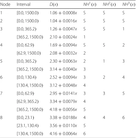
5.2 Tandem nine-node network
Figure 3 shows a nine-node tandem sample network over which we have simulated the PFA_SPF algorithm.
The transmission rate of the wireless link between any nodesiandjabove is 11 Mbps if the nodes are one hop apart, 5.5 Mbps if they are two hops apart, 2 Mbps if they are three hops apart, and 1 Mbps if they are four hops apart. For the nodes that are more than four hops apart, there is no wireless link.
The simulation of PFA_SPF algorithm for the network in Fig. 3 generates the next-hop node entriesNH1(x)and distance functions for each node, as tabulated in Table 1.
The path setup mechanism minimizing the hop count results in the next-hop entriesNH2(x)as shown in Table 1.
In addition, a path setup mechanism that is optimized with respect to a packet size of 1500 bytes generates the next-hop entriesNH3(x).
Throughput gains of the PFA_SPF algorithms over the minimum hop Dijkstra algorithm and the Dijkstra algo-rithm with a fixed packet size of 1500 bytes are shown in Fig. 4. The average throughput gain over the minimum hop Dijkstra algorithm is up to 70 % and increases as the packet size grows. The maximum throughput gain is up to 130 % and is even more significant. The throughput gain over the Dijkstra algorithm with a fixed packet size of 1500 bytes is only significant when the packet size is less than 400 bytes. It provides up to 25 and 60 % gains for average and maximum throughputs, respectively.
5.3 Random networks
In this section, we generate random networks with vari-ous node sizes over a circular area in which the nodes are distributed randomly.
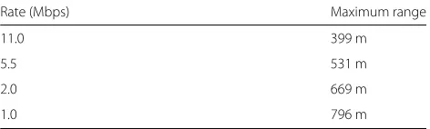
The range-to-rate mapping for the wireless links in the networks is based on the range-to-rate values presented in [23, 24], which are tabulated in Table 2.
S 1 2 3 4 8
5.5 Mb/s
11 Mb/s
2 Mb/s
1 Mb/s
Fig. 3Nine-node tandem sample network
Table 1The results of algorithms for tandem nine-node network
Node Interval D(x) NH1(x) NH2(x) NH3(x)
1 [0.0, 1500.0) 1.06+0.0008x S S S
2 [0.0, 1500.0) 1.04+0.0016x S S S
3 [0.0, 365.2) 1.26+0.0047x S S 1
[365.2, 1500.0) 2.10+0.0024x 1
4 [0.0, 62.9) 1.69+0.0094x S S 2
[62.9, 1500.0) 2.08+0.0032x 2
5 [0.0, 365.2) 2.30+0.0063x 2 1 3
[365.2, 1500.0) 3.14+0.0040x 3
6 [0.0, 130.4) 2.52+0.0094x 3 2 4
[130.4, 1500.0) 3.12+0.0048x 4
7 [0.0, 62.9) 2.95+0.0141x 3 3 5
[62.9, 365.2) 3.34+0.0079x 4 [365.2, 1500.0) 4.18+0.0056x 5
8 [0.0, 23.1) 3.38+0.0188x 4 4 6
[23.1, 130.4) 3.56+0.0110x 5 [130.4, 1500.0) 4.16+0.0064x 6
An example of a random network of 30 nodes is shown in Fig. 5. Note that the center node is indicated by a cir-cle, and that the rest of the nodes are indicated with cross marks. Figure 6 shows the link rates between each pair of nodes for this network.
For those nodes that are separated by more than 796 m, there is no link possible. Consequently, there is no guaran-tee that a randomly generated network will beconnected; i.e., each node can be reached from another one by a connection path. We exclude those networks that are not connected from our discussion.
0 100 200 300 400 0
10 20 30 40 50 60
Packet Size (byte)
Throughput Gain over Dijkstra (x=1500) (%)
Average Gain Max. Gain
0 500 1000 1500 0
20 40 60 80 100 120 140
Packet Size (byte)
Throughput Gain over Min−hop Dijkstra (%)
Average Gain Max. Gain
Table 2Wireless link rate values for ranges
Rate (Mbps) Maximum range
11.0 399 m
5.5 531 m
2.0 669 m
1.0 796 m
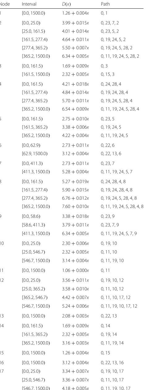
For this particular example, the PFA_SPF algorithm gen-erated the paths and overall distance functions from each node to the center node, as shown in Table 3.
As the packet size increases, the algorithm favors the paths with higher MAC layer overhead time but with higher overall transmission rates. The nodes that are far away from the center node are more likely to have more than one path than the ones closer to the center node. Figure 7 shows this phenomenon clearly for various net-work sizes.
To obtain the plots in this section, we generated 1000 connected random networks for each network size.
For nodes with multiple paths, the intervals are par-titioned at small packet sizes; in the earlier particu-lar example, there are 10 partition points: 25.0, 58.6, 62.9, 161.5, 277.4, 365.2, 411.3, 468.5, 545.7, and 546.7. This partitioning is also observable in the general case, as shown in Fig. 8 for 80-node randomly generated networks.
Another interesting metric is the number of paths per node for various network sizes. As it can be seen in Fig. 9, as the network becomes more crowded, the number of paths for a node increases because the number of alter-native paths increases. In Fig. 10, the average number of paths for a node shows this trend more clearly.
0 500 1000 1500 2000 2500 3000 3500 0
Fig. 5An example network with 30 nodes
The performance of the PFA_SPF algorithm is simulated along with the minimum hop Dijkstra algorithm and the Dijkstra algorithm with fixed packet size of 1500 bytes. The average throughput gains of the PFA_SPF algorithm over these algorithms are shown in Fig. 11. As seen in Fig. 11, the average gains of our solution over the mini-mum hop count method and the Dijkstra algorithm opti-mized for 1500 bytes are computed as up to more than 100 and 30 %, respectively. The throughput average is taken over all nodes, except the center node, for an ensemble of 1000 random networks. These plots show that the per-formance of the fixed packet size Dijkstra algorithm is almost identical to the PFA_SPF algorithm large packet sizes around 1500 bytes, and that the PFA_SPF algorithm provides modest gains for small packet sizes. Except for very small packet sizes, the PFA_SPF algorithm provides better performance than does the minimum hop Dijk-stra algorithm, because the latter ignores the MAC layer overheads and link rates.
Figure 12 shows the average of the maximum gains for a network at a particular packet size. The maximum gains are computed for all nodes of a network, except the cen-ter node, and then those maximum values are averaged over 1000 randomly generated networks. The gains of our solution over the minimum hop count method and the Dijkstra algorithm optimized for 1500 bytes are computed as up to 300 and 100 %, respectively.
In extreme cases, the PFA_SPF algorithm can provide even larger throughput gains, as indicated in Fig. 13. Here, we compute the maximum gains for an ensemble of 1000 networks at a particular packet size. Our generic solu-tion outperforms the minimum hop count method and the Dijkstra algorithm optimized for 1500 bytes by up to 450 and 250 %, respectively. Note that some curves are not visible because they overlap with other curves.
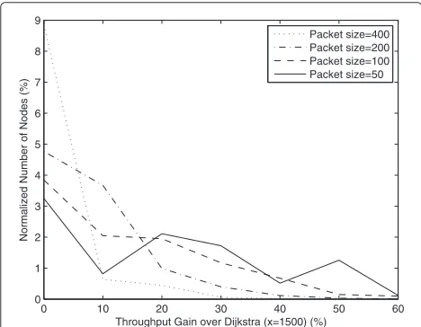
Figure 14 shows the normalized histogram of nodes vs. the percentage of the throughput gain over the Dijkstra
0 1000 2000 3000 0
Table 3The results of PFA_SPF algorithm for sample network
Node Interval D(x) Path
1 [0.0, 1500.0) 1.26+0.004x 0, 1
2 [0.0, 25.0) 3.99+0.015x 0, 23, 7, 2
[25.0, 161.5) 4.01+0.014x 0, 23, 5, 2 [161.5, 277.4) 4.64+0.011x 0, 19, 24, 5, 2 [277.4, 365.2) 5.50+0.007x 0, 19, 24, 5, 28, 2 [365.2, 1500.0) 6.34+0.005x 0, 11, 19, 24, 5, 28, 2
3 [0.0, 161.5) 1.69+0.009x 0, 3
[161.5, 1500.0) 2.32+0.005x 0, 15, 3
4 [0.0, 161.5) 4.21+0.018x 0, 24, 28, 4
[161.5, 277.4) 4.84+0.014x 0, 19, 24, 28, 4 [277.4, 365.2) 5.70+0.011x 0, 19, 24, 5, 28, 4 [365.2, 1500.0) 6.54+0.009x 0, 11, 19, 24, 5, 28, 4
5 [0.0, 161.5) 2.75+0.010x 0, 23, 5
[161.5, 365.2) 3.38+0.006x 0, 19, 24, 5 [365.2, 1500.0) 4.22+0.004x 0, 11, 19, 24, 5
6 [0.0, 62.9) 2.73+0.011x 0, 22, 6
[62.9, 1500.0) 3.12+0.004x 0, 22, 13, 6
7 [0.0, 411.3) 2.73+0.011x 0, 23, 7
[411.3, 1500.0) 5.28+0.004x 0, 11, 19, 24, 5, 7
8 [0.0, 161.5) 5.27+0.019x 0, 24, 28, 4, 8
[161.5, 277.4) 5.90+0.015x 0, 19, 24, 28, 4, 8 [277.4, 365.2) 6.76+0.012x 0, 19, 24, 5, 28, 4, 8 [365.2, 1500.0) 7.60+0.010x 0, 11, 19, 24, 5, 28, 4, 8
9 [0.0, 58.6) 3.38+0.018x 0, 23, 9
[58.6, 411.3) 3.79+0.011x 0, 23, 7, 9 [411.3, 1500.0) 6.34+0.005x 0, 11, 19, 24, 5, 7, 9
10 [0.0, 25.0) 2.30+0.006x 0, 19, 10
[25.0, 546.7) 2.32+0.005x 0, 11, 10 [546.7, 1500.0) 3.14+0.004x 0, 11, 19, 10
11 [0.0, 1500.0) 1.06+0.000x 0, 11
12 [0.0, 25.0) 3.56+0.011x 0, 19, 10, 12
[25.0, 365.2) 3.58+0.010x 0, 11, 10, 12 [365.2, 546.7) 4.42+0.007x 0, 11, 10, 17, 12 [546.7, 1500.0) 5.24+0.006x 0, 11, 19, 10, 17, 12
13 [0.0, 1500.0) 2.08+0.003x 0, 22, 13
14 [0.0, 161.5) 1.69+0.009x 0, 14
[161.5, 365.2) 2.32+0.005x 0, 19, 14 [365.2, 1500.0) 3.16+0.003x 0, 11, 19, 14
15 [0.0, 1500.0) 1.26+0.004x 0, 15
16 [0.0, 1500.0) 3.12+0.004x 0, 22, 13, 16
17 [0.0, 25.0) 3.34+0.007x 0, 19, 10, 17
[25.0, 546.7) 3.36+0.007x 0, 11, 10, 17 [546.7, 1500.0) 4.18+0.005x 0, 11, 19, 10, 17
Table 3The results of PFA_SPF algorithm for sample network Continued
18 [0.0, 1500.0) 2.30+0.006x 0, 15, 18
19 [0.0, 365.2) 1.26+0.004x 0, 19
[365.2, 1500.0) 2.10+0.002x 0, 11, 19
20 [0.0, 58.6) 2.95+0.014x 0, 1, 20
[58.6, 1500.0) 3.36+0.007x 0, 15, 18, 20
21 [0.0, 1500.0) 2.52+0.009x 0, 1, 21
22 [0.0, 1500.0) 1.04+0.001x 0, 22
23 [0.0, 468.5) 1.69+0.009x 0, 23
[468.5, 1500.0) 4.22+0.004x 0, 11, 19, 24, 23
24 [0.0, 161.5) 1.69+0.009x 0, 24
[161.5, 365.2) 2.32+0.005x 0, 19, 24
[365.2, 1500.0) 3.16+0.003x 0, 11, 19, 24
25 [0.0, 1500.0) 2.08+0.003x 0, 22, 25
26 [0.0, 545.7) 1.69+0.009x 0, 26
[545.7, 1500.0) 4.20+0.004x 0, 11, 19, 24, 26
27 [0.0, 25.0) 3.99+0.015x 0, 19, 10, 27
[25.0, 62.9) 4.01+0.014x 0, 11, 10, 27
[62.9, 546.7) 4.40+0.008x 0, 11, 10, 17, 27
[546.7, 1500.0) 5.22+0.007x 0, 11, 19, 10, 17, 27
28 [0.0, 161.5) 2.95+0.014x 0, 24, 28
[161.5, 277.4) 3.58+0.010x 0, 19, 24, 28 [277.4, 365.2) 4.44+0.007x 0, 19, 24, 5, 28 [365.2, 1500.0) 5.28+0.004x 0, 11, 19, 24, 5, 28
29 [0.0, 161.5) 3.99+0.015x 0, 15, 18, 29
[161.5, 1500.0) 4.62+0.011x 0, 15, 18, 20, 29
algorithm with fixed packet size of 1500 bytes. When the packet size is large, the histogram is accumulated around 0 because most nodes do not have any significant through-put gain. As the packet size gets smaller, the histogram gets wider and flatter because more nodes have through-put gain. The means of these histograms are the same as the corresponding average throughput gains shown in Fig. 11. Likewise, Fig. 15 shows the normalized his-togram of nodes vs. the percentage of the throughput gain over the minimum hop Dijkstra algorithm. In contrast to Fig. 14, the histogram gets wider and flatter, as the packet size gets larger. Thus, the higher gains of the PFA_SPF algorithm occur for larger packet sizes as shown in Fig. 11.
6 Conclusions
0 200 400 600 800 1000 1200 1400 1600 1800
Distance from the center node (m)
Average number of paths per node
20 Nodes 40 Nodes 60 Nodes 80 Nodes
Fig. 7Average number of paths vs. distance from the center node
0 500 1000 1500
0
Histogram of Interval Partition Points (%)
Fig. 8Histogram of interval partition points for 80-node networks
1 1.5 2 2.5 3 3.5 4 4.5 5 5.5 6
Probablity Mass Funtion of Nodes
20 Nodes 40 Nodes 60 Nodes 80 Nodes
Fig. 9Probability mass function of nodes vs. number of paths
20 30 40 50 60 70 80
Average Number of Paths
Fig. 10Average number of paths vs. network size
0 200 400 600
Average Throughput Gain over Dijkstra (x=1500) (%)
20 Nodes 40 Nodes 60 Nodes 80 Nodes
0 500 1000 1500 0
Average Throughput Gain over Min−hop Dijkstra (%)
20 Nodes 40 Nodes 60 Nodes 80 Nodes
Fig. 11Average throughput gain of the PFA_SPF algorithm
0 500 1000 1500 0
Average Max. Throughput Gain over Dijkstra (x=1500) (%)
20 Nodes 40 Nodes 60 Nodes 80 Nodes
0 500 1000 1500 0
Average Max. Throughput Gain over Min−hop Dijkstra (%)
20 Nodes 40 Nodes 60 Nodes 80 Nodes
0 500 1000 1500 0
50 100 150 200 250
Packet Size (byte)
Maximum Throughput Gain over Dijkstra (x=1500) (%)
20 Nodes 40 Nodes 60 Nodes 80 Nodes
0 500 1000 1500 0
50 100 150 200 250 300 350 400 450 500
Packet Size (byte)
Maximum Throughput Gain over Min−hop Dijkstra (%)
20 Nodes 40 Nodes 60 Nodes 80 Nodes
Fig. 13Maximum throughput gain of the PFA_SPF algorithm
scalar but a function of packet parameters such as packet size. As can be seen in the algorithm statement, there is no assumption of any specific network model. That is, the algorithm is not limited to a specific MAC layer, physical layer, or a network model. In fact, the algo-rithm can be used both in multi-hop wired and wireless networks.
In this paper, we aim to present the basic novel algo-rithm as well as the benefits of the algoalgo-rithm over a fun-damental and basic network model and compare it with the most used classical base path setup metrics: hop count and optimized for only 1500 bytes. The results show the significant potential benefits for the future routing proto-cols leveraging and integrating such a packet size-aware path setup algorithm.
0 10 20 30 40 50 60
0 1 2 3 4 5 6 7 8 9
Throughput Gain over Dijkstra (x=1500) (%)
Normalized Number of Nodes (%)
Packet size=400 Packet size=200 Packet size=100 Packet size=50
Fig. 14Normalized histogram of nodes vs. throughput gain over Dijkstra (x=1500) for 80-node networks
0 50 100 150 200
0 0.5 1 1.5 2 2.5 3
Throughput Gain over Min−Hop Dijkstra (%)
Normalized Number of Nodes (%)
Packet size=50 Packet size=200 Packet size=600 Packet size=1500
Fig. 15Normalized histogram of nodes vs. throughput gain over minimum hop Dijkstra for 80-node networks
In particular, we simulated the algorithm for the packet size-aware path setup that we show to significantly improve the overall performance with respect to the prior work.
The effect of the proposed path setup mechanism pre-sented in this paper on the performance of higher layer protocols, such as transport layer protocols, in particular TCP, is known and left as a future work. Especially, TCP performance getting adversely affected by out-of-order packet delivery is within the scope of the future work of this study as our method can generate multiple paths for a single TCP connection.
However, as mentioned in the introduction part of the paper, there are various research on TFRC (TCP-friendly rate control) with multi-path routing protocols along with the coding techniques (e.g., digital fountain codes) where our proposed method/algorithm in this paper can be an integral part of the solution. In such solutions, the adverse effects of wireless packet losses and out-of-order packet delivery to the TFRC-based transport protocol are elim-inated while still avoiding the congestion collapse in the network.
Even though in this paper, we have done an initial anal-ysis based on a real but relatively small network. As a future work, we plan to experiment and simulate with larger networks along with other 802.11 standards such as 802.11 n/g/a and to model the link delay and throughput along with the larger packet sizes, such as Jumbo frames. In addition, we plan to design and implement a com-plete routing protocol minimizing the total transmission delay and/or the total energy consumption based on the proposed generic algorithm and test it over real network deployments along with extensive simulations.
Competing interests
Authors’ information
Mustafa Arisoylu received the PhD degree from University of California San Diego (UCSD), in Electrical and Computer Engineering in 2006. He received his MS and BS degrees from Bilkent University, Turkey, both in Electrical Engineering in 1999 and 2001, respectively. Dr. Arisoylu conducted research on resource allocation and performance optimization in communication networks and authored several publications. In 2004, he was a visiting researcher at Los Alamos National Laboratory, (LANL). Dr. Arisoylu worked as a researcher at Cal-IT2 (California Institute for Telecommunications and Information Technology), designing and architecting advanced multi-hop wireless mesh networks for emergency response applications. Dr. Arisoylu joined a startup spinoff company from Cal-IT2 / UCSD, at its seed stage where he served as Research Scientist and Vice President of Research and Development. He later joined the systems design group at Ericsson Inc. Research and Development Center in Boulder, Colorado. Currently, he is serving as a Senior Engineering Manager R&D at system architecture group at Ericsson Silicon Valley Research and Development Center in San Jose, CA.
Received: 18 December 2015 Accepted: 4 February 2016
References
1. X Wu, W Li, F Liu, H Yu, inIEEE International Conference on Wavelet Active
Media Technology and Information Processing (ICWAMTIP). Packet size distribution of typical Internet applications, (2012)
2. C Fraleigh, S Moon, B Lyles, C Cotton, M Khan, D Moll, R Rockell, T Seely,
C Diot, Packet-level traffic measurements from the Sprint IP backcone.
IEEE Network.17(6), 6–16 (2003)
3. R Sinha, C Papadopulos, J Heidemann, Internet packet size distributions:
some observations, ISI-TR-2007-643. USC/Information Sciences Institute Technical Report, (2007)
4. Y Cheng, V Ravindran, A Leon-Garcia, in26th IEEE International Conference
on Computer Communications, INFOCOM. Internet traffic characterization using packet-pair probing, (2007)
5. J Downey, Understanding VoIP packet sizing and traffic engineering, in
SCRE Cable-tec Expo, White Paper, (June 2005)
6. K Thompson, G Miller, R Wilder, Wide-area internet traffic patterns and
characteristics. IEEE Network.11(6), 10–23 (1997)
7. A Mena, J Heidemann, inNineteenth Annual Joint Conference of the IEEE
Computer and Communications Societies, INFOCOM. An empirical study of real audio traffic, (2000)
8. Sun, Jun, Y Wen, L Zheng, inProceedings IEEE International Conference on
Computer Communications, INFOCOM. On file-based content distribution over wireless networks via multiple paths: coding and delay trade-off, (2011)
9. JW Byers, M Luby, M Mitzenmacher, A digital fountain approach to
asynchronous reliable multicast. IEEE Journal on Selected Areas in
Communications, JSAC.20(8), 1528–1540 (2002)
10. JW Byers, M Lubyy, M Mitzenmacher, A Rege, inProc. Special Interest Group
on Data Communications Conference ACM SIGCOMM. A digital fountain approach to reliable distribution of bulk data, (1998)
11. S Floyd, et al., inProceedings of Special Interest Group on Data
Communications Conference, ACM SIGCOMM. Equation-based congestion control for unicast applications (Sweden, Stockholm, 2000), pp. 43–56
12. J Padhye, D Kurose, R Towsley, inProc. Int’l. Wksp. Network and Op. Sys.
Support for Digital Audio and Video, NOSSDAV. A model based TCP-friendly rate control protocol, (1999)
13. S Cen, PC Cosman, GM Voelker, End-to-end differentiation of congestion
and wireless losses. Netw. IEEE/ACM Trans.11(5), 703–717 (2003)
14. M Arisoylu, T Javidi, RL Cruz, inIEEE International Conference on
Communications, ICC. End-to-end and MAC-layer fair rate assignment in interference-limited wireless access networks, (2006)
15. C Kim, Y Ko, NH Vaidya, inIEEE Military Communications Conference,
MILCOM. Link-state routing protocol for multi-channel multi-interface wireless networks, (2008)
16. M Heusse, F Rousseau, GB Sabbatel, A Duda, inTwenty-Second Annual
Joint Conference of the IEEE Computer and Communications, INFOCOM. Performance anomaly of 802.11b, (2003)
17. P Liu, Z Tao, S Panwar, inIEEE International Conference on Communications,
ICC. A cooperative MAC protocol for wireless local area networks, (2005)
18. T Korakis, S Narayanan, A Bagri, S Panwar, inIEEE International Conference
on Communications, ICC. Implementing a cooperative MAC protocol for wireless LANs, (2006)
19. J Dunn, M Neufeld, A Sheth, D Grunwald, J Bennett, inIEEE First
International Conference on Broadband Networks, BroadNets. A practical cross-layer mechanism for fairness in 802.11 networks, (2004) 20. DSJ De Couto, D Aguayo, J Bicket, R Morris, A high throughput path
metric for multi-hop wireless routing. Journal Wireless Networks - Special
issue: Selected papers from ACM MobiCom 2003.11(4), 419–434 (2005)
21. M Arisoylu, S Ergut, RL Cruz, R Rao, inIEEE Consumer Communications and
Networking Conference, CCNC. Packet size aware path setup for wireless networks, (2008)
22. C Pepin, UC Kozat, AS Ramprashad, in4th International Symposium on
Modeling and Optimization in Mobile, Ad Hoc and Wireless Networks, IEEE WiOpt. A joint traffic shaping and routing approach to improve the performance of 802.11 mesh networks, (2006)
23. B Awerbuch, D Holmer, H Rubens, High throughput route selection in multi-rate ad hoc wireless networks, Wireless On-demand Network Systems (WONS), (2004)
24. DHB Awerbuch, H Rubens, The medium time metric: High throughput route selection in multirate ad hoc wireless networks. Mobile Networks
and Applications.11(2), 253–266 (2006)
25. M Arisoylu, RL Cruz, T Javidi, inProceedings of the Allerton Conference on
Communications, Control, and Computing. Rate assignment in micro-buffered high speed networks, (2005)
26. R Perlman,Interconnections: bridges, routers, switches and Internet-working
protocols, 2nd Ed. (Addison Wesley, 1999)
27. D Bertsekas, R Gallager,Data Networks, 2nd edn. (Prentice Hall,
Englewood Cliffs, New Jersey, 1992)
28. J Moy, OSPF version 2, RFC 2328 (1998). http://ietf.org/rfc/rfc2328.txt 29. T Clausen, P Jacquet, A Laouiti, P Minet, P Muhlethaler, A Qayyum, L
Viennot. (Optimized link state routing protocol, draft MANET-IETF, 2002). http://www.ietf.org/internet-drafts/draft-ietfmanet-olsr-07.txt 30. D Oran, OSI IS-IS Intra-domain routing protocol, RFC 1142 (1990). http://
ietf.org/rfc/rfc1142.txt
31. J Moy,OSPF, Anatomy of an Internet Routing Protocol. (AddisonWesley,
Boston, 1998)
32. R Murty, J Padhye, R Chandra, A Wolman, B Zill, inNSDI ’08: 5th USENIX
Symposium on Networked Systems Design and Implementation. Designing high performance enterprise Wi-Fi networks, (2008)
33. A Raniwala, T Chiueh, inIEEE International Conference on Computer
Communications INFOCOM. Architecture and algorithms for an IEEE 802.11-based multi-channel wireless mesh network, (Miami, FL, 2005)
34. KN Ramachandran, EM Belding, KC Almeroth, MM Buddhikot, inIEEE
International Conference on Computer Communications INFOCOM. Interference-aware channel assignment in multi-radio wireless mesh networks, (2006)
35. R Sivakumar, P Sinha, V Bharghavan, CEDAR: a core-extraction distributed
ad hoc routing algorithm. IEE J. Selected Areas Commun.17(8),
1454–1465 (1999)
36. A Raha, SS Babu, MK Naskar, O Alfandi, Hogrefe D, inIEEE 5th International
Conference on Advanced Networks and Telecommunication Systems (ANTS). Trust integrated link state routing protocol for wireless sensor networks (TILSRP), (2011)
37. EC van der Meulen, Three-terminal communication channels. Adv. Appl.
Probab.3, 120–154 (1971)
38. A Sendonaris, E Erkip, B Aazhang, User cooperation diversity—Part I:
system description. IEEE Trans. Commun.51(11), 1927–1938 (2003)
39. A Sendonaris, E Erkip, B Aazhang, User cooperation diversity—Part II: implementation aspects and performance analysis. IEEE Trans. Commun. 51(11), 1939–1948 (2003)
40. T Cover, A Gamal, Capacity theorems for the relay channel. IEEE Trans. Inf.
Theory.25(5), 572–584 (1979)
41. G Kramer, M Gastpar, P Gupta, Cooperative strategies and capacity
theorems for relay networks. IEEE Trans. Inf. Theory.51(9), 3037–3063
(2005)
42. A Host-Madsen, Capacity bounds for cooperative diversity. IEEE Trans. Inf.
Theory.52(4), 1522–1544 (2006)
43. L Lai, K Liu, H El Gamal, The three-node wireless network: achievable rates
44. DSJD Couto, D Aguayo, J Bicket, R Morris, in9th annual international conference on mobile computing and networking (ACM MobiCom 03). A high-throughput path metric for multi-hop wireless networks, (2003)
45. D Aguayo, J Bicket, S Biswas, G Judd, R Morris, inProceedings of Special
Interest Group on Data Communications Conference, ACM SIGCOMM. Link-level measurements from an 802.11b mesh network, (2004)
46. R Draves, J Padhye, B Zill, inProceedings of Special Interest Group on Data
Communications Conference, ACM SIGCOMM. Comparison of routing metrics for static multi-hop wireless networks, (2004)
47. A Adya, P Bahl, J Padhye, A Wolman, L Zhou, inIEEE International
Conference on Broadband Networks, BroadNets. A multi-radio unification protocol for ieee 802.11 wireless networks, (2004)
48. S Keshav, inProceedings of Special Interest Group on Data Communications
Conference, ACM SIGCOMM. A control-theoretic approach to flow control, (1991)
49. R Draves, J Padhye, B Zill, inannual international conference on mobile
computing and networking in ACM MobiCom. Routing in multi-radio, multi-hop wireless mesh networks, (2004)
50. R Karrer, A Sabharwal, E Knightly, inACM Workshop on Hot Topics in
Networks (HotNets). Enabling large-scale wireless broadband: the case for TAPs, (2003)
51. D Aguayo, J Bicket, S Biswas, DD Couto, inannual international conference
on mobile computing and networking MobiCom Poster. MIT roofnet: construction of a production quality ad-hoc network, (2003)
52. K Ramachandran, I Sheriff, E Belding, K Almeroth, inPAM’07 Proceedings of
the 8th international conference on Passive and active network measurement. Routing stability in static wireless mesh networks, (2007)
53. K Fall, inProceedings of Special Interest Group on Data Communications
Conference, ACM SIGCOMM. A delay-tolerant network architecture for challenged Internets, (2003)
54. Y Zeng, et al., Directional routing and scheduling for green vehicular
delay tolerant networks. Wireless Netw.19(2), 161–173 (2013)
55. T Spyropoulos, et al., Routing for disruption tolerant networks: taxonomy
and design. Wireless Netw.16(8), 2349–2370 (2010)
56. A Vasilakos, et al.,Delay tolerant networks: Protocols and applications. (CRC
Press, Boca Raton, 2012)
57. A Dvir, et al., Backpressure-based routing protocol for DTNs. ACM
SIGCOMM Comput. Commun. Rev.41(4), 405–406 (2011)
58. Li Peng, et al., inIEEE International Conference on Computer
Communications INFOCOM. CodePipe: an opportunistic feeding and routing protocol for reliable multicast with pipelined network coding, (2012)
59. Li Peng, et al., Reliable multicast with pipelined network coding using opportunistic feeding and routing. IEEE Trans. Parallel Distributed Syst. 25(12), 3264–3273 (2014)
60. L Liu, et al., Physarum Optimization: A biology-inspired algorithm for the
Steiner tree problem in networks. IEEE Trans. Comput.64(3), 819–832
(2015)
61. Y Liu, et al., Multi-layer clustering routing algorithm for wireless vehicular
sensor networks. IET Commun.4(7), 810–816
62. C Busch, et al., Approximating congestion + dilation in networks via
“Quality of Routing” games. IEEE Trans. Comput.61(9), 1270–1283 (2012)
63. T Meng, et al., Spatial reusability-aware routing in multi-hop wireless networks. IEEE TMC (2015). doi:10.1109/TC.2015.2417543
64. Y-S Yen, et al., Flooding-limited and multi-constrained QoS multicast routing based on the genetic algorithm for MANETs. Math. Comput.
Modell.53(11-12), 2238–2250 (2011)
65. M Youssef, et al., Routing metrics of cognitive radio networks: a survey.
IEEE Commun. Surv. Tutorials.16(1), 92–109 (2014)
66. I Woungang, SK Dhurandher, A Athanasios, V Vasilakos,Routing in
opportunistic networks. (Springer, 2013)
67. XM Zhang, et al., Interference-based topology control algorithm for delay-constrained mobile ad hoc networks. IEEE Trans. Mobile Comput. 14(4), 742–754 (2015)
68. A Attar, et al., A survey of security challenges in cognitive radio networks:
solutions and future research directions. Proc. IEEE.12, 3172–3186 (2012)
69. AV Vasilakos, et al., Information centric network: research challenges and
opportunities. J. Netw. Comput. Appl.52, 1–10 (2015)
70. Marwaha S, et al., inCongress on Evolutionary Computation, CEC.
Evolutionary fuzzy multi-objective routing for wireless mobile ad hoc networks, vol. 2, (2004), pp. 1964–1971
71. A Vasilakos, et al., Optimizing QoS routing in hierarchical ATM networks using computational intelligence techniques. IEEE Transactions on Systems, Man, and Cybernetics, Part C: Applications and Reviews, (2003)
72. W Quan, C Xu, AV Vasilakos, J Guan, H Zhang, LA Grieco, inIFIP Networking
Conference. TB2F: Tree-bitmap and bloom-filter for a scalable and efficient name lookup in content-centric networking, (2014)
73. K Liu, et al., A cooperative MAC protocol with rapid relay selection for
wireless ad hoc networks. Comput. Netw.91, 262–282 (2015)
74. L Xiang, et al., in8th Annual IEEE Communications Society Conference on
Sensor, Mesh and Ad Hoc Communications and Networks (SECON). Compressed data aggregation for energy efficient wireless sensor networks, (2011)
75. C Perkins, Royer E, inSecond IEEE Workshop on Mobile Computing Systems
and Applications, WMCSA. Ad hoc on-demand distance vector routing, (1999)
76. DB Johnson, DA Maltz, Dynamic source routing in Ad-hoc Wireless Networks. Mobile Computing, pages 153–181. Kluwer Academic Publishers (1996)
Submit your manuscript to a
journal and benefi t from:
7 Convenient online submission
7 Rigorous peer review
7 Immediate publication on acceptance
7 Open access: articles freely available online
7 High visibility within the fi eld
7 Retaining the copyright to your article