R E S E A R C H
Open Access
Environment-Adaptable Fast
Multi-Resolution (EAF-MR) optimization in
large-scale RF-FPGA systems
Minhee Jun
*†, Rohit Negi
†, Shihui Yin, Mohamed Alawieh, Fa Wang, Megha Sunny, Tamal Mukherjee
and Xin Li
Abstract
Software-defined radio (SDR) can have high communication quality with a reconfigurable RF front-end. One of the main challenges of a reconfigurable RF front-end is finding an optimal configuration among all possible configurations. In order to efficiently find an optimal configuration, Environment-Adaptable Fast (EAF) optimization utilizes calculated signal-to-interference-and-noise ratio (SINR) and narrows down the searching space (Jun et al., Environment-adaptable efficient optimization for programming of reconfigurable Radio Frequency (RF) receivers, 2014). However, we found several limitations for applying the EAF optimization to a realistic large-scale Radio Frequency-Field Programmable Gate Array (RF-FPGA) system. In this paper, we first investigated two estimation issues of RF impairments: a saturation bias of nonlinearity estimates and limited resources for RF impairment estimation. Using the estimated results, the SINR formula was calculated and used for the Environment-Adaptable Fast Multi-Resolution (EAF-MR) optimization, which was designed by applying the EAF optimization to multi-resolution optimization. Finally, our simulation set-up demonstrated the efficiency improvement of the EAF-MR optimization for a large-scale RF-FPGA.
Keywords: Software-defined radio (SDR), Reconfigurable RF front-end, Large-scale RF-FPGA, Estimation of RF impairments, Environment-Adaptable Fast Multi-Resolution (EAF-MR) optimization
1 Introduction
Wireless communication is ubiquitous in our daily life using an excessive number of communication standards: 3G/4G/LTE cellular service, Wi-Fi, bluetooth, and so on. The new paradigm of Internet of Things (IoT) has also accelerated the plethora of wireless communication [3]. The abundance of communication standards has recently increased interest in cognitive radio because its multi-standard platform supports cost reduction of service sup-pliers and the efficient use of frequency spectrum.
First, cognitive radio allows for more affordable ser-vice to providers and subscribers. Previously, when a new communication standard comes out, service providers have spent a huge amount of expenditure for building a new infrastructure such as base stations and hardware
*Correspondence:[email protected] †Equal contributors
Department of Electrical and Computer Engineering, Carnegie Mellon University, Pittsburgh, PA 5000 Forbes Ave, Pittsburgh, 15213 PA, USA
systems corresponding to a new communication standard. Particularly in rural areas, it is a burdensome and time-consuming process for service suppliers to include rural areas to the new service coverage due to a low user den-sity. However, cognitive radio must have multi-standard platforms in its hardware. Due to the dynamic property of cognitive radio, service providers can reuse the existing infrastructures when serving a new communication stan-dard. Thus, service providers reduce the expensive cost and time for distributing the infrastructure for the new standard.
In addition, cognitive radio is an optimal solution for handling inefficient radio frequency (RF) spectrum uti-lization. The RF spectrum is a limited natural resource, and it is officially managed by Federal Communications Commission (FCC) [1]. Given the fixed standard assign-ment policy of governassign-ment agencies, issues might arise for future wireless communication due to the excessive amount of communication standards. Since the RF spec-trum occupation rate has a wide variation, in time and
space, from 15 to 85% [1], cognitive radio can dynamically and intelligently change its communication channel and temporally utilize the portions of the unused RF spectrum (called a spectrum hole or white space) [7,8,17].
This multi-standard platform of cognitive radio is achieved by implementing software-defined radio (SDR). In order to design the SDR architecture, there have been studies to design fixed wide-band RF front-end. The fixed wide-band RF front-end accommodates various signals on different RF spectrum bands by choosing a homo-dyne architecture. Also, the fixed wide-band RF front-end generally requires to remove RF filters and to choose durable RF components with wide-band signals [6]. How-ever, the condition of wide-band signals limits the choice of RF components and performance. In contrast, a recon-figurable RF front-end (also called reconrecon-figurable Radio Frequency-Field Programmable Gate Array (RF-FPGA)) is more appropriate for the SDR architecture in terms of selectivity and sensitivity [9].
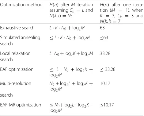
The reconfigurable RF front-end is a novel RF front-end concept recently proposed by the U.S. Defense Advanced Research Projects Agency (DARPA) [5]. The RF-FPGA replaces with the fixed wideband RF front-end but it is combined with the the classical baseband RF-FPGA [4,14]. Meanwhile, a reconfigurable RF front-end can be programmed to switch its RF components: there are var-ious RF component banks, including amplifier, filter, and mixer banks as given in Fig. 1 [2, 16]. The details of RF-FPGA architectures are introduced in [12,13].
This architecture of RF-FPGA as shown in Fig.1 max-imizes the reconfigurability of SDR, and thus, RF-FPGA is an attractive alternative for supporting a multi-standard platform of cognitive radio in the future. Particularly, the enhanced reconfigurability in this RF-FPGA archi-tecture is directly related to increasing the reusabil-ity of this device. The RF-FPGA reusabilreusabil-ity can save
hardware re-design cost for updating wireless communi-cation standards. In addition, RF-FPGA can have a high performance solving the practicality issue of a cognitive radio because it can be dynamically tunable to a particular setting optimized to real-time communication environ-ments in the field.
Note that RF-FPGA operates on RF spectrums, and thus, it is distinguished from digital FPGA that operates on baseband spectrums. It is known that RF-FPGA is ben-eficial with respect to reduced life cycle cost, reduced re-design cost, and service for multiple DoD platform.
RF-FPGA can dynamically adapt to the communication environment on-the-fly retaining a high communication quality. RF-FPGA is defined as a dynamically reconfig-urable (programmable) RF transceiver. RF-FPGA is com-posed of an array of reconfigurable RF component blocks that can have as many as 100 bits of control. As shown in Fig.1, the RF component blocks are adjusted by switches that are deployed between the RF component blocks. The switches connect the RF component blocks that are cho-sen by the reconfiguration engine while bypassing the RF component blocks in the idle mode (i.e., the bypassed RF component blocks are not selected by the reconfig-uration engine). This RF-FPGA architecture is designed to maximize the flexibility of RF-FPGA for adapting to varying RF environments. This flexibility of RF-FPGA can allow to change the operating frequency band of the RF transceiver.
A reconfigurable RF front-end can flexibly select one of the RF components arranged in each component bank using switches and serially connect them in differ-ent architectures, including heterodyne and homodyne [5]. The ability to have many configurations in compo-nent banks supports a multi-standard platform for cur-rently existing standards. The component bank needs to include a number of configurations with different ranges
to consider future standards. For future standards, the component banks contain many configurations that may not be accounted for current settings. When a reconfig-urable RF front-end selects RF components in the com-ponent banks, it aims to satisfy the requirements of the given communication standard. Thus, a reconfigurable RF front-end supports a multi-standard platform by dynam-ically changing its occupying RF spectrum of various standards for cognitive radio.
In order to operate a reconfigurable RF front-end, an important challenge is finding an optimal configura-tion among all possible configuraconfigura-tions (a configuraconfigura-tion is mapped to a combination of RF components in a reconfig-urable RF front-ends). In order to find the configuration, an optimization problem is defined as finding a config-uration that minimizes its cost function (such as power consumption) while satisfying constraint requirements of a given communication standard (such as signal-to-noise ratio (SNR)) [9]. Studies have aimed to solve this opti-mization problem in a reconfigurable RF front-end. Tao et al.’s study in [15] proposed two-phase relaxation opti-mization that attempts to reduce the possibility of find-ing local optimal configurations. This process performs local relaxation optimization in two separate phases: In the first phase, the optimization finds a configuration of the highest SNR; in the second phase, starting from the found configuration, the optimization searches an optimal point using the relaxation optimization. This optimiza-tion has improved selectivity of optimal configuraoptimiza-tion, and thus, when the reconfigurable radio is initially pro-grammed, several base configurations (i.e., default con-figurations) can be pre-programmed into it, based on the desired communication standards. However, it has a limited capability of reducing reconfiguration load for a dynamic communication environment, with blockers and large interferers appearing randomly at different fre-quencies. In this case, the reconfigurable RF front-end cannot be pre-programmed exhaustively, since there are too many possible scenarios to be considered. Rather, a fast algorithm to adapt the RF front-end to interfer-ers in real-time is needed. Thus, a fast optimization algorithm—called Environment-Adaptable Fast (EAF) optimization—was proposed for speeding up the opti-mization of a reconfigurable RF front-end in a dynamic spectrum environment [9].
The EAF optimization improves its optimization effi-ciency by predicting configurations that are less likely to pass the communication quality requirement of a given standard. The prediction is performed based on signal-to-interference-and-noise ratio (SINR), which is calculated—as opposed to simulated —using RF impairment informa-tion. These are three steps of the EAF optimization: (1) RF impairments should be estimated when a recon-figurable RF front-end is manufactured. The estimators
of RF impairments are designed based on the signal model of baseband signals. For RF impairment infor-mation, the estimation methods of RF impairments are designed as presented in [9–11]. (2) The SINR calcula-tion formula for the EAF optimizacalcula-tion is described in [11]. In the SINR calculation, impairing signal power due to each of the RF impairments—phase noise, IIP3, noise figure—was separately derived in terms of the power of the signal of interest and interference. The SINR calculation uses estimated RF impairments and a signal spectrum in a given communication environ-ment. Thus, real-time blocker information is reflected in SINR calculations. (3) Finally, the EAF optimization uses the SINR calculation to identify the configurations that likely do not meet a SINR specification and to nar-row down the search space of configurations. The EAF optimization method was shown to reduce the computa-tional cost significantly, finding an optimal configuration after only five iterations instead of searching all possible configurations exhaustively. Therefore, the EAF optimiza-tion method can be successfully utilized as a heuris-tic to find a minimum power configuration of adequate SNR in an experimental case of a small reconfigurable RF system.
In contrast, a large-scale RF-FPGA poses a significant problem for the EAF optimization. A realistic RF-FPGA is likely to be controlled by several hundred bits that select the component values. In such a large-scale RF-FPGA, it is not possible to directly measure and characterize the RF impairments of each of the possible configurations.
In order to utilize thelarge-scale RF-FPGA for cogni-tive radio, our research focused on developing an efficient algorithm, called Environment-Adaptable Fast Multi-Resolution (EAF-MR) method. The EAF-MR method has the following contributions:
(1) RF impairment estimation in a large-scale RF-FPGA : we propose a method that estimates unknown RF impairments of the configurations that can not directly estimated using baseband signals in a large-scale RF-FPGA. The configurations with known estimates are used to measure other
configurations with unknown RF impairments. This estimation method is useful because only a limited number of configurations in a large-scale RF-FPGA are estimated due to limited time and computation resources.
(3) the improved time-efficiency of EAF-MR
optimization algorithm for a large-scale RF-FPGA : in the EAF-MR algorithm, the EAF optimization synergizes with the multi-resolution method in order to improve the time efficiency of the optimization process in a large-scale RF-FPGA.
In this paper, we investigate a model-based approach to solve this problem in order to use the EAF optimiza-tion in large-scale RF-FPGA systems. First, we studied RF impairment estimation for a large-scale RF-FPGA system. We derived statistical signal models of RF impairments, and based on the statistical signal models, we designed estimators of RF impairments. We focused on two main problems while applying the estimators of RF impair-ments to a large-scale RF-FPGA system: two saturation areas of nonlinearity estimates and limited resources in RF impairment estimation procedures. The saturation areas of nonlinearity estimates are caused by a wide range of RF front-ends. In order to solve the saturation, we designed a formula for changing the transmission signal power in an estimation procedure. Also, we considered limited resources in RF impairment estimation in a large-scale RF front-end. Solving the limited resource prob-lem, we used a design of experiments (DoE) approach that effectively selects sample configurations among the large number of all possible configurations in a large-scale RF-FPGA. We also used an interpolation method that obtains unknown component values from known component values of RF impairments calculated from sample configurations. Second, we derived a formula that calculates SINR in a given communication environment in terms of phase noise, nonlinearity, and noise figure. In order to improve the accuracy of the SINR calcula-tion, the impairing signal power by each RF impairment was separately analyzed considering the frequency off-set of interference and the power of the signal of interest and interference. We assumed that RF impairments are estimated, and a signal spectrum is obtained by a sig-nal asig-nalyzer [9], a configuration of reconfigurable RF front-ends that bypasses all filters and amplifiers. Third, using the SINR calculation, we designed the EAF-MR optimization method that hastens an optimization pro-cess for finding an operable configuration in a large-scale RF-FPGA system. Simulation results showed that our EAF-MR optimization method significantly improves its optimization speed compared with the multi-resolution optimization method.
Now, we clarify the terminologies that will be frequently used in the following context:
• component: the element—such as amplifier, filter, or mixer—that composes a reconfigurable RF front-end. The components are placed and switched in RF component banks.
• configuration: a cascade of the chosen components from RF component banks in a reconfigurable RF front-end. Configurations can be reconfigured by switching each component.
• overall RF impairment: the metric that represents the overall RF impairment of a configuration.
• component value: the metric that represents the RF impairment of a component.
2 RF impairment estimation in large-scale
RF-FPGA systems
In this section, we investigate the estimation of RF impair-ments in alarge-scaleRF front-end. RF impairments in a RF system are described in [16], and the basic insight of signal processing is explained in [1,2,8,9]. The first prob-lem associated with this large scale is that the large num-ber of RF front-ends span a wide range of RF impairment values. Due to the wide range of RF impairment values, the RF front-end is very likely to experience saturation in an estimation process when transmission power is fixed. In Section2.1, we solve this problem by designing a method that adjusts the transmission power during the estima-tion procedure. The second problem is the large number of configurations in a large-scale RF front-end. This prob-lem is tackled by using a design of experiments (DoE) approach and an interpolation procedure as discussed in Section2.2. These methods are important in a large-scale RF front-end because we cannot simulate (or estimate) all configurations; we can only simulate a limited number of sample configurations. For example, a reconfigurable RF front-end with 63 bits of control means that the num-ber of configurations is about 9.2 × 10¹⁸, which results in an impractically time-consuming estimation procedure. Our methods of RF impairment estimation in a large-scale RF front-end are utilized to efficiently extract unknown properties of RF components from known properties that are calculated from simulated data. This method of RF impairment estimation is applied to a large-scale RF front-end of 63 bits.
2.1 Tackling a wide range of RF impairment values: bias in IIP3estimate
Consider a large-scale RF-FPGA system, as shown in Fig. 2. This example large-scale RF-front-end has three amplifiers with 21 bits of control. This front-end has 63 bits of control, allowing a wide range of values for gain and the third-order input intercept points (IIP3). This is defined in terms of the ratio of the first order gain over the third order gain. Due to this, configurations with a wide range of IIP3values are possible.
Fig. 2An example of a large-scale RF-FPGA system with 63 bits of control: each of three tunable amplifiers in (a) has 21 bits of control. Each tunable amplifier with 21 bits of control is composed of three cascaded tunable amplifiers with 7 bits of control as shown in (b)
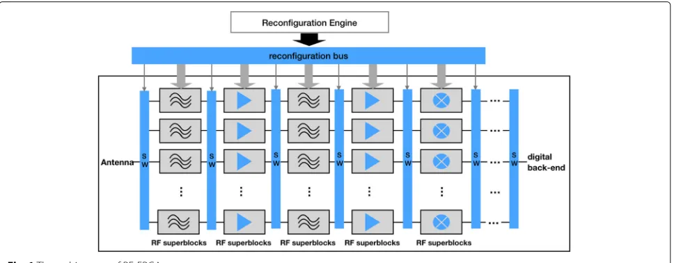
estimated IIP3from−80 to−10 dBm is mainly due to high gains obtained by passing through multiple ampli-fiers. In order to solve the bias (saturation) problem in IIP3 estimation, we obtained a formula for adjusting transmis-sion power to a RF front-end. The transmistransmis-sion powerPtx was derived from the upper and lower boundaries of IIP3 saturation.
The upper boundary of IIP3saturation is related to ther-mal noise. Therther-mal noise power should be sther-maller than the intermodulated signal power of transmitted signals in order to be detected during the estimation procedure. More specifically, the overall thermal noise power after passing a reconfigurable RF front is given asNF0(dBm/Hz)+ f(dB)+NF(dB)where thermal noise floor isNF0 (dBm/Hz)=
Fig. 3Calculated IIP3from library data is given on thex-axis and estimated IIP3from simulation is given on they-axis when three amplifiers are
reconfigured in a reconfigurable RF front-end. There are two saturation areas according to where the IIP3estimate is: the lower boundary around
−174(dBm/Hz),f(dB)=10·log10B(dB)for the bandwidth B(Hz)of the transmitted signal, andNF(dB)is an additional noise figure for noise margin. Meanwhile, the intermod-ulated signal with IIP3 has a power of 3·Psig(dBm)−2· IIP3 (dBm) where Psig is the nominal transmitted signal power of the two transmitted signals that are intermod-ulated. So, we derive the following condition to allow accurate estimation of IIP3.
NF0 (dBm/Hz)+f(dB)+NF(dB)<3·Psig(dBm)−2·IIP3(dBm), (1)
wheref(dB)=10·log10B(dB).
From this, the upper boundary of IIP3saturation is given as,
The lower boundary of IIP3saturation in Fig.3is related to the transmitted signal powerPsig. A transmitted signal with a high power level suffers from nonlinearity inter-modulation. When an intermodulated signal by the third order nonlinearity has a power as large as the power of a transmitted sinusoid, the transmission power is defined as IIP3. Thus, the transmitted signal powerPsigshould be smaller than IIP3as follows,
Psig(dBm)<IIP3(dBm). (3)
From (2) and (3), the range of IIP3over which we can expect low bias is given as,
K0 < IIP3(dBm) < K0 + K, (4)
Now, we specify the choice of transmission power Ptx(dBm) =Psig(dBm)+P(dB)that should be used for IIP3 estimation to allow low bias.
The overall IIP3of a configuration of cascaded compo-nents is as follows,
From this, we can assume that the nonlinearity of
the last cascaded component is dominant, i.e., 1 IIP3 ≈
Now, we assume that the approximate range of IIP3such as IIP3,N(min) and IIP3,N(max) of (the last) component is known. We define the transmission power increase P over the nominal valuePsig(dBm)for use in IIP3estimation. Then, the range of power increasePthat satisfies (6) is given as follows,
P(min)(dB)in order to avoid IIP3estimation saturation.
P(dB)=mean Thus, in a large-scale RF front-end, the transmission powerPtxfor IIP3estimation is given as,
Ptx(dBm)=Psig(dBm)+P(dB)
=0.5·(IIP3,N(min)(dBm)+IIP3,N(max)(dBm)) −0.5·K−G1N−1(dB). (9)
2.2 Tackling a large number of configurations: DoE and interpolation methods
A significant challenge in applying the EAF optimization method to a large-scale RF front-end is that RF impair-ment estimation is time-consuming when the number of configurations is very large. In this section, we use model-based design of experiments (DoE) and interpo-lation methods to drastically reduce the time needed for estimation.
2.2.1 Configuration subsets: full-factorial design set, screening design set, and sample configuration set
The configurations of a large-scale RF front-end can be successively narrowed into the following subsets: full-factorial design set, screening design set, and sample configuration set as shown in Fig.4.
Fig. 4Configuration subsets—full-factorial design set, screening design set, and sample configuration set
design set is a subset of the full-factorial design set and includes the most significant factors of configurations. The configurations of a screening design set are obtained by reconfiguring only a few of the most significant bits (MSBs) of sub-amplifiers as seen in Fig.5. In our exam-ple, two MSBs of three sub-amplifiers are allowed to be reconfigured with the remaining bits held constant at 0, resulting in a screening design set of configurations with 18 bits of control. Finally,sample configurationsare selected for actual simulation and data collection from within the screening design set.
2.2.2 Configuration subsets and RF impairment calculation
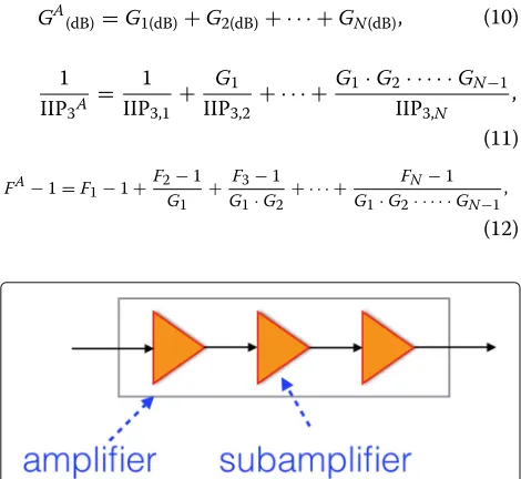
In a cascaded chain of RF components, as in Fig.2, we can calculate the overall RF impairment from the component values using the following formula,
GA(dB)=G1(dB)+G2(dB)+ · · · +GN(dB), (10)
1 IIP3A =
1 IIP3,1+
G1
IIP3,2 + · · · +
G1·G2· · · · ·GN−1 IIP3,N
,
(11)
FA−1=F1−1+F2−1 G1 +
F3−1 G1·G2+ · · · +
FN−1 G1·G2· · · · ·GN−1,
(12)
Fig. 5Three sub-amplifiers in an amplifier- In our example, two MSBs of three sub-amplifiers are allowed to be reconfigured for a screening design set
where Gk, IIP3,k, and Fk are the gain, IIP3, and noise factor, respectively, of the kth component of a configu-ration (k = 1, 2,· · ·,N), and GA, IIP3A, andFA are the overall gain, IIP3, and noise factor, respectively, of the configuration.
Thus, in order to obtain an unknown value of overall RF impairments, we need to obtain the component values of RF impairments. We will now explain how to obtain component values from sample configurations and how to select sample configurations based on a linear model of RF components in Section2.2.3.
2.2.3 Linear model of RF impairments in a large-scale RF-FPGA
We note that, perhaps surprisingly, (10), (11), and (12) are all of the same general linear form,
Z=h1X1+h2X2+ · · · +hkXk+ · · · +hNXN, (13)
whereXkrepresents the RF impairment of thekth compo-nent of a configuration,hkis a coefficient for thekth term, k = 1, 2,· · ·,N, andZrepresents the overall RF impair-ment of the configuration. The impairimpair-ment can be either gain (Xk = Gk(dB)), IIP3(Xk = 1/IIP3), or noise factor
(Xk =Fk−1). For example, for (11),Xk = 1
IIP3,k,h1=1, hk=G1·G2· · · · ·Gk−1, fork∈ {2,· · ·,N}.
When the value of the kth component Xk is chosen in a set of component values, {θk,1,θk,2,· · ·,θk,Ck}, we can define the vectorθ that is composed of all available component values as follows,
θ=
θ1,1,θ1,2,· · ·,θ1,C1
,θ2,1 ,θ2,2,· · ·,θ2,C2,· · ·,θN,1 ,θN,2,· · ·,θN,CN T
.
(14)
Then, we can build a linear model,
Y=H·θ+N, (15)
whereYis the vector of measured RF impairment using simulation or actual measurement (each element corre-sponding to one sample configuration that is simulated) while the vectorNrepresents measurement noise during the estimation process.
We will now present how to define the matrixHin (15). Thekth componentXkin (13) chooses a component value θk,k in (14)(k ∈ {1, 2, 3,· · ·,Ck}), and (13) is given as follows,
Y=h1θ1,1+h2θ2,2+ · · · +hkθk,k· · · +hNθN,N+N
=h1·g1,h2·g2,· · ·,hk·gk,· · ·,hN·gN
·θ
=h·θ (16)
(gk)1,l=
1 ifl=k
0 otherwise,. (17)
wherel=1, 2, 3,· · ·,Ck.
Thus, we can define the matrixHin (15) composed of the row vectorhin (16) corresponding to the measured sample configurationY.
Based on (15), we obtain the unknown characteristicsθ of all components using least-squares (LS) estimation as below,
θ =HT·H −1
·H·Y. (18)
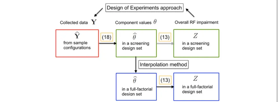
Given any configurations with unknown RF impair-ment, we can use (13) to estimate its impairment using the estimated component values θ. Thus, using a screening design set of sample configurations, we can estimate com-ponent valuesθand use the method (13) to predict the RF impairments of any configurations as shown in Fig.6.
2.2.4 DoE for choosing optimal sample configurations
We select a set ofoptimalsample configurations among the configurations in the screening design set using the design of experiments (DoE) approach. The DoE method selects an optimal set ofmsample configurations (equiv-alently, the matrix H in (18) corresponding to the m selected sample configurations) using a D-optimal design approach. In the matrixH, each row corresponds to one of sample configurations. The D-optimal design approach iteratively updates a set of sample configurations in order to increase the determinant |HT ·H|, i.e., minimize the log-determinant of noise variance matrix in (15) to find optimal sample configurations. The matrixHis updated until its conditional number—the ratio of the maximal eigenvalue of H over the minimal eigenvalue of H—is small. The condition of a small conditional number pre-vents an error inYfrom causing a large error inθ in15
The implementation details of the DoE method for choos-ing sample configurations are described in Algorithm 1 (Appendix).
2.2.5 Simulation results
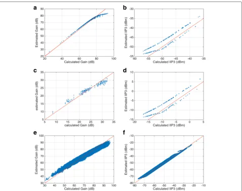
Figure 7 shows the simulation results of gain and IIP3 estimation by applying the DoE method to the RF-FPGA (Fig. 2). We verify that the method can be successfully used to estimate RF impairments of any configuration using a model-based approach, with component values estimated by a DoE method.
The estimated gain and IIP3,Y in (18), of sample con-figurations are plotted on they-axis against true gain and IIP3Yof the sample configurations on thex-axis in Fig.7a andbrespectively. The simulation results show that the estimates of Y proportionally increase with true values ofY. (At high gain values, around 100 dB, the estimates begin to saturate in Fig.7a. Also, configurations where at least one amplifier is bypassed have IIP3estimates which are about 3 dB lower in Fig.7b.)
The estimated gain and IIP3,θ of the three amplifiers, are plotted on they-axis against true gain and IIP3θof the three amplifiers on thex-axis in Fig.7canddrespectively. The estimatesθ proportionally increase with true values ofθ. (The estimated IIP3of the first and second amplifiers are about 3 dB lower than that of the third amplifier in Fig.7d.)
Finally, the estimated gain and IIP3,Z, of the remain-ing configurations in the screenremain-ing design set are plotted on they-axis against true gain and IIP3Zon thex-axis in Fig.7eandfrespectively. The estimatesZproportionally increase with true values ofZ.
2.2.6 Interpolation method
In order to extend the RF impairments estimated for con-figurations in the screening design set to the full-factorial
Fig. 7Simulation results for RF impairment estimation using the design of experiments (DoE) method.aEstimated gainYˆof configurations in a sample configuration set.bEstimated IIP3Yˆof configurations in a sample configuration set.cEstimated gainθˆof each amplifier.dEstimated IIP3θˆ
of each amplifier.eEstimated gainZˆof configurations in a screening design set.fEstimated IIP3Zˆof configurations in a screening design set
design set, the interpolation method is applied. Recollect that the configurations in the screening design set only use a few of the most significant bit (MSB) bits of each com-ponent, with the other bits frozen to zero. The assumption made here is that the bits of each component define a real number (or set of real numbers) and that the true RF impairment is a continuous function of this (set of ) real numbers.
The red data points shown in Fig. 8—the configura-tions in a screening design set—have identified valuesθin (18) obtained from the sample configurations as described in Section 2.2.4. The stared points—the configurations in a full factorial design set—have unknown but identi-fiable values by applying the interpolation method. First, the parameters in a mathematical model are determined to fit data of configurations in a screening design set to the mathematical model. Second, using the parameters
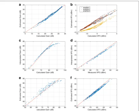
and the mathematical model, the interpolation method interpolates the unknown component values in config-urations. The pseudocode of the interpolation method is given in Algorithm 2. For the interpolation process, we utilized the natural neighbor interpolation. Simulation results of applying the interpolation method are plotted in Fig. 9. Thus, we could measure configurations in a full-factorial design set from a screening design set.
The gain and IIP3 characteristics of amplifiers in the full-factorial design set on the y-axis are obtained by applying the interpolation method to the corresponding estimators of the screening design set. Figure9a,b, which shows gain and IIP3respectively on they-axis, shows close agreement with the true values on thex-axis.
Fig. 8The interpolation method is applied to obtain information of the configurations with known RF impairments from the configurations with unknown RF impairments
using the formula (10), (11), and (12). The calculated over-all gain and IIP3of 150 configurations in a full factorial set on they-axis are plotted against the true values on thex -axis in Fig.9c,drespectively while estimates of gain and IIP3 obtained by simulation of the same configurations representing a full-factorial set are plotted in Fig.9e,f. The results demonstrate that unknown RF impairments of the configurations in a full factorial design set are successfully obtained by applying the interpolation method.
2.2.7 Efficiency of the design of RF impairment estimation for a large-scale RF-FPGA
In this section, we discuss how the design of RF impair-ment estimation for a large-scale RF-FPGA improves the efficiency of RF impairment estimation. The designed DoE and interpolation methods are applied to measure RF impairment in a large-scale RF front-end of 63 bits from sample configuration data. In Table1, the number of simulations (runs) and the required estimation time are calculated for three configuration sets: a full-factorial design set, a screen designing set (of reconfiguring two MSBs of knobs), and a sample configuration set. The sim-ulation time required for the estimation of gain is 41 s while IIP3 is 42 s. The number of configurations to be simulated is about 1019, 2.6 × 10⁵, and 384 in a full-factorial design set, a screening design set, and a sample configuration set, respectively. The total required simu-lation time is about 1.3 × 10¹³ years, 3 × 10³ h, and 4.4 h, respectively. We found that while estimating RF impairments for a full-factorial or screening design set is costly and time-consuming, estimating RF impairments for sample configurations are powerful and cost-effective, as shown in the Table1. Thus, we verify that the design
of RF impairment estimation for a large-scale RF-FPGA is important to utilize limited resources, such as time and power, for estimation.
3 SINR calculation in a large-scale RF-FPGA
The signal-to-interference-and-noise ratio (SINR) of a configuration is calculated as described in [11] and given as below,
SINR= PS
Pphn+Pip3+Pn
, (19)
Table 1Comparison of time consumption for RF impairment estimation
RF impairments Gain IIP3
Simulation running time 41 s 42 s
for a configuration
The number of simulations 1019runs 1019runs for full-factorial designs
The number of simulations 2.6×10⁵runs 2.6×10⁵runs for screening designs (2 MSBs of
components are reconfigured)
The number of simulations for 384 runs 384 runs sample configurations
Total simulation time for 1.3×10¹³years 1.33×10¹³years
full factorial designs
Total simulation time for 3×10³h 3.1×10³h
screening designs
Fig. 9Simulation results of the interpolation method.aInterpolated gain of an amplifier.bInterpolated IIP3of an amplifier.cEstimated gain of a
configuration with three amplifiers using interpolated gain.dEstimated IIP3of a configuration with three amplifiers using interpolated IIP3.
eEstimated gain of a configuration using simulation.fEstimated IIP3of a configuration using simulation
where PS is the signal power,Pphn, Pip3, andPn are the impairing signal powers caused by phase noise ment, nonlinearity impairment, and thermal noise impair-ment, respectively.
For the SINR calculation in a large-scale RF front-end, we combined the previous estimation methods of RF impairments for obtaining Pphn and Pip3 and our new approach to extend the estimation methods to a large-scale RF front-end. ThePphn andPip3in the SINR calculation can be calculated from the estimation meth-ods of RF impairments introduced in [9–11]. Using the estimation methods, the parameters of RF impairments were directly obtainable for all available configurations of a small-scale reconfigurable RF front-end. However, the designed methods cannot be utilized in a large-scale reconfigurable RF front-end due to the limitation of time resource as discussed in Section4.3. Thus, for the SINR
calculation in a large-scale reconfigurable RF front-end, we use the estimated RF impairments obtained by apply-ing the DoE approach and the interpolation method. The details of the designed estimation method of RF impair-ments for a large-scale reconfigurable RF front-end were introduced in Section 2.2.
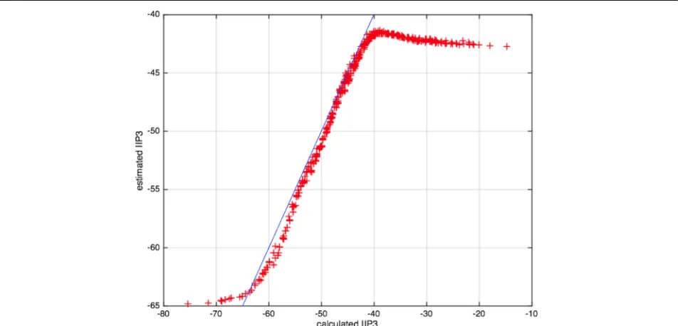
Fig. 10SINR calculated using (10) in [11]ascenario 1: interference of the power−30 dBm at 20 MHz frequency offset from the signal of interest of−67 dBm andbscenario 2: two interferences of the power
−35 dBm at 150 and 300 MHz frequency offset, respectively, from the signal of interest of−67 dBm
4 EAF-MR optimization in a large-scale RF-FPGA
4.1 Optimization problem in a large-scale RF-FPGA The optimization problem for searching an optimal con-figuration in a small-scale reconfigurable RF front-end was previously defined in [9–11] as follows,
min F(x),
xs.t.gk(x)≥Gkfor 1≤k≤K
(20)
where the vector-valuedxindicates one of the available configurations for a reconfigurable RF front-end, and each element of xrepresents the parameter value of an indi-vidual component.F(x)is a cost function such as power consumption of x, which needs to be minimized, while gk(x) ≥ Gk (1 ≤ k ≤ K) describe constraints such as SINR.
However, this optimization model in (20) is not suit-able to describe the optimization problem in a large-scale reconfigurable RF front-end due to the explosively
increased size of search space. With the increased search space in a large-scale reconfigurable RF front-end, the lim-ited time resource causes a bottleneck for a practical use of the previously suggested optimization methods. Practi-cally, the amount of time consumed to obtain SINR using simulation (or measurement) in an optimization process dramatically increases in a large-scale reconfigurable RF front-end. Thus, one of the important factors to be con-sidered in a large-scale reconfigurable RF front-end is reducing the number of simulations (or measurements) for obtaining SINR in an optimization process.
Including this search space factor (e.g., the number of simulations), we now define the optimization problem in a large-scale reconfigurable RF front-end with a new cost functionF(x)+H(n)as follows,
min F(x)+H(n), xs.t.gk(x)≥Gkfor 1≤k≤K
(21)
whereH(n)is a function of the suggested total numbern of simulations (or measurements) in a given optimization algorithm. In our example of a large-scale RF front-end with 63 bits of control, the optimization problem in (21) is given by defining thatF(x)is the power consumption of the configurationx,g1(x)is the SINR ofx,G1is the SNR threshold of the given communication standard,K = 1, andH(n)is given aslog2(n).
We note that according to the choice of optimization algorithms, an optimal configurationxthat satisfies the optimization problem in (21) can vary because there is a trade of the costsF(x)andH(n). If a designed algorithm runs more iterations of algorithms to find an optimal con-figuration, the cost of F(x) decreases but the costH(n) increases, and vice versa. Thus, the optimal configurations of different optimization algorithms may not be the same according to how to design the algorithms.
Solving the defined optimization problem, we introduce the Environment-Adaptable Fast Multi-Resolution (EAF-MR) optimization designed for a large-scale RF-FPGA to adapt to the dynamic conditions in communication.
4.2 EAF-MR optimization
We designed the EAF-MR optimization method [9] by applying the EAF optimization that utilizes the SINR calculation to the multi-resolution optimization.
The multi-resolution optimization improve the two-phase relaxation optimization for a large-scale reconfig-urable RF front-end. The multi-resolution optimization narrows down the search space into screening design sets of available configurations in a large-scale RF front-end. The size of screening design sets is determined by the number of active reconfiguration knob bits in all RF components. The fewer active bits of knobs, the more sparsely the characteristic values of the config-urations in the screening design sets are distributed. The multi-resolution optimization tries to search for two types of configurations in the two phases, from small to large active bits. If there is no improvement for one cycle of iterations for all configurations, the iterative reconfiguration is stopped. The pseudocode of the multi-resolution algorithm is given in Algorithm 3 (Appendix).
In our EAF-MR optimization method, we applied the primary algorithmic structure of the multi-resolution optimization, and we utilized the calculated SINR in order to reduce the number of configurations to be simulated. When the SINR calculation of the config-urations does not meet the pre-defined SINR thresh-old, the configurations are trimmed out in the list of configurations to be simulated. The pseudocode of the multi-resolution algorithm is given in Algorithm 4 (Appendix).
4.3 Search space of optimization methods
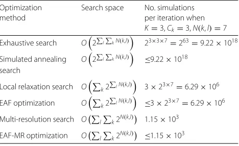
In numerical experiments, we focus only on the multi-resolution optimization and the EAF-MR optimization instead of including traditional optimization methods: exhaustive search, simulated annealing search, local relax-ation search (the details of these traditional optimizrelax-ation methods are described in [9]). However, the neces-sary search space for configurations in a large-scale RF front-end is too big to include these traditional optimization algorithms in Table2. Assume that a large-scale RF front-end has K reconfigurable(tuable) com-ponents, and its kth component has the lth compo-nent values of N(k,l) bits where l ∈ {1, 2,· · ·,Ck} and k ∈ {1, 2,· · ·,K}. The search space of exhaustive search is given as O(kl2N(k,l)) = O(2k
lN(k,l)). Simulated annealing search also has a search space of O(2k 7 bits of control in Fig. 5. In this example, the num-ber of simulations per one iteration of exhaustive search, simulated annealing search, local relaxation search, and multi-resolution search are 9.22×10¹⁸,≈ 9.22×10¹⁸, O(6.29 × 10⁶), and O(1.15 × 10³), respectively (dur-ing this one iteration a series of cascaded components
Table 2Search space of optimization methods
Optimization Search space No. simulations
method per iteration when
Simulated annealing O2l
in a large-scale RF front-end is reconfigured only once).
The EAF optimization and the EAF-MR optimization have the same search space as the local relaxation and the multi-resolution search, respectively. However, these optimization methods reduce the search spaces by elim-inating candidate configurations that have SINR calcula-tion under a threshold. The size of reduced search space depends on the communication environment in a field.
Reducing search space is a critical factor in the optimization of a large-scale RF front-end due to prac-tical time consumption. For this reason, it is impracprac-tical to apply classical methods to a large-scale RF front-end. However, the search space is dramatically reduced from exponential increase in exhaustive search to lin-ear increase in multi-resolution slin-earch in terms of the number of configurations and the number of components as shown in Table 2. Therefore, multi-resolution search and the EAF-MR optimization method are practically applicable in a large-scale RF front-end.
Table3shows the upper bounds ofH(n)in (21) assum-ingCkandN(k,l)are given asLandN0respectively. We can observe that the upper bound ofH(n)is significantly reduced in multi-resolution search and the EAF-MR opti-mization in terms of the base 2 logarithms. Also, Table3 shows an example case ofH(n)after one iteration when K = 3, Ck = 3, and N(k,l) = 7. The observed val-ues prove that multi-resolution search and the EAF-MR optimization significantly reduceH(n)in (21) from 63 to 10.17. It demonstrates that the two optimization methods are the most efficient to minimize the cost functionF(x)+ H(n)presented in (21). Thus, in order to search the opti-mal configuration of reconfigurable RF front-end when solving the optimization problem in (21), multi-resolution and the EAF-MR optimization are the algorithms of our interest, and thus are focused in simulation.
Table 3H(n)in (21) of optimization methods
Optimization method H(n)afterMiteration assumingCk =Land
We finally demonstrate the performance of our EAF-MR optimization using a Matlab simulation.
4.4.1 Simulation setting
We verified the performance of the designed EAF-MR optimization in a large-scale RF-FPGA (Fig.2) using Mat-lab Simulink. In the simulation, we used the commu-nication standard IEEE 802.11g, and the required SNR specification is 11.5 dB. The transmitted signals have the bandwidth 20 MHz and the power− 67 dBm. The RF-FPGA has 63 bits, which implies approximately 1019 configurations. There are two fixed RF filters, one fixed IF filter, and three 21 bit amplifiers. The power consump-tion range of all possible configuraconsump-tions is from 11.85 to 107.85 mW. We tested two optimization methods, multi-resolution and EAF-MR, on the scenario, which has one interferer of−30 dBm at 20 MHz frequency offset from the signal of interest.
4.4.2 Simulation results
Tables4and5show the simulation results of the multi-resolution search and the EAF-MR optimization. While the multi-resolution optimization method took 2172 sim-ulations for finding an optimal configuration, our EAF-MR optimization method required only two simulations. The EAF-MR optimization increases optimization effi-ciency since it is able to discard a large number of con-figurations whose calculated SINR does not satisfy the SNR specification. As shown in Table5, multi-resolution search took 816 and 1356 simulations in phase 1 and phase 2, respectively, whereas the MR-EAF optimization needed 1 and 1 simulation in phase 1 and phase 2, respectively.
Both optimization methods found optimal configura-tions that satisfy the SNR specification (11.5 dB) as shown in Table5. In terms of power consumption, we found that
Table 4Simulation results of no. simulations
Optimization Phase I Phase II Total number
method of simulations
Multi-resolution optimization 816 1356 2172
MR-EAF optimization 1 1 2
there is a trade-off between higher power consumption and the number of simulations. The power consump-tion of the EAF-MR’s optimal configuraconsump-tion is around 21 mW compared to around 12 mW (multi-resolution’s optimal configuration). The power consumption of the EAF-MR’s optimal configuration is almost twice of that of multi-resolution search. However, the maximal power consumption of all possible configurations is larger than 100 mW. Compared to the maximal power consumption, the EAF-MR optimization found an optimal configuration that has a power consumption in a reasonable range of energy efficiency.
The simulation results verify that our EAF-MR opti-mization method is appropriately designed for a large-scale reconfigurable RF front-end to perform fast reconfigura-tion in dynamic communicareconfigura-tion environments. Table 6 shows that the cost function of the MR-EAF optimization in the optimization problem (21) is significantly improved compared to that of the multi-resolution search. Although the two optimization methods give two different optimal configurations, the cost function in (21) is dropped with the MR-EAF optimization because it needs only a few reconfigurations to find the optimal one.
5 Conclusion
In this paper, we investigated the application of the EAF optimization in a large-scale RF-FPGA. To estimate RF impairments in a large-scale RF front-end, we solved two main problems. First, we solved the saturation of non-linear estimates due to a wide range of RF front-ends. To avoid the saturation problem, we obtained a formula for adjusting transmission power for an estimation pro-cedure. Second, we solved a limited estimation resources problem. Because of a large number of configurations, it is not possible to directly measure and characterize the RF impairments of all possible configurations. We extended the estimation procedure to a large-scale RF-FPGA using the design of experiments (DoE) approach and the interpolation method. Finally, we designed an
Table 5Simulation results of optimization
Optimization Power (mW) SINR (dB) Total number
method of simulations
Multi-resolution optimization 12.52 11.63 2172
Table 6Simulation results and cost function in the optimization problem (21)
Optimization F(x) H(n) F(x)+H(n)
method
Multi-resolution optimization 12.52 11.08 33.60
MR-EAF optimization 20.98 1 21.98
EAF multi-resolution (EAF-MR) optimization method in which the EAF optimization method was applied to a multi-resolution (MR) optimization. Simulation results showed that our EAF-MR optimization requires only two iterations while multi-resolution optimization takes more than 2000 iterations. There is a trade-off between efficiency and local optimum. However, as an optimal configuration exists, finding a global optimum is not nec-essary. The main focus of our research is attaining low computational cost (fast convergence) in optimization for a real-time application. Therefore, using this algo-rithm, reconfigurable RF front-ends can move forward to a reliable multi-standard platform for the needs of future communication systems.
In the future, we want to investigate spectral strategies that help to prune the space of RF configurations to be explored (“search space”) and rules to automatically rank preferred RF configurations. In order to narrow down the search space, we plan to study the heuristic rules that are applicable using the reconfigurability of filters and local oscillators (LOs). While reconfiguring filters and LOs, we assume that the characteristics of RF components (e.g., filters’ center frequency and bandwidth) and also the sig-nal spectrum are accessible. When a blocker appears, in order to improve communication quality, in addition to the choice of filters, etc., we can also change either radio frequency (RF) or intermediate frequency (IF) of the RF system based on the blocker information in the signal spectrum. For example, the blocker signal can be effec-tively eliminated if it is placed on the stopband of a notch filter in the frequency domain. In order to satisfy this condition, the IF of a reconfigurable RF front-end can be changed by reconfiguring LOs considering the char-acteristics of the notch filter. The heuristic strategies for reconfiguring filters and LOs will help a reconfigurable RF front-end improve the speed of an optimization process in dynamic communication environments.
Appendix
In line1,mis the number of sample configurations to be selected from a screening design set given in the matrix XScreeningin order to estimate RF impairments.XScreening is a row matrix composed of all configurations in a screen-ing design set that is obtained by reconfigurscreen-ing a few pre-defined MSBs of sub-amplifiers. In line 3,HScreeningis
Algorithm 1 The DoE Approach: find XDoE (a set of sample configurations) and a matrixHDoEin (15).
1: INPUT:m,XScreening
2: Ncondition= ∞ conditional number
3: whileNcondition>Ncondition(threshold)do
4: XDoE=functiond-optimal method
Ncondition(threshold) is a constant of the maximal limit of condition numberNcondition.
In line 1,Xtest,Xknown, andVknownare a matrix that indi-cates a set of test configurations, a set of configurations with known component values, and a set of the known component values inXknown, respectively. In the for-loop, the valuesvtestof each componentxtestare interpolated on theith component—separately in the cascaded order—of configurationsVtest.vknowncorresponds toθ in (14), and
xknownhas the indices of the known component values in a full-factorial set. The interpolation is performed based on the known component valuesvknownandxknownusing natural neighbor interpolation.
In Algorithm 3,x(current), SNR(current), Power(current) rep-resent a current configuration, the simulated SNR, and power of the current configuration, respectively. nBit1
Algorithm 2 The Interpolation Approach: estimate unknown component valuesVtestfor test configurations
Vtestin a full factorial set.
1: INPUT:Xtest,Xknown,Vknown
2: N ← the number of components in the configura-tions ofXtest
3: fori=1, 2, 3,· · ·,Ndo
4: xknown ←thei-th cascaded component of a con-figuration ofXknown
5: xtest ←thei-th cascaded component of the con-figurations ofXtest
6: vknown←component values corresponding toXp. it is obtainable fromVknown
7: vtest←functioninterpolation(xknown,vknown,xtest)
8: Vtest(i)←vtest
Algorithm 3Multi-Resolution Algorithm
5: while(there has been recent updates onx(current)) do
6: c ← the next available component of the current componentc
7: X←a set of configurations obtained by recon-figuring the componentcwithnbits of control while other components are fixed.
8: SNR(x) ← simulated (or measured) SNR for
∀x∈X
20: while(there has been recent updates onx(current)) do
21: c ← the next available component of the
current componentc
22: X←a set of configurations obtained by recon-figuring the componentcwithnbits of control while other components are fixed.
23: SNR(x) ← simulated (or measured) SNR for ∀x∈X
30: else if(cis a component in an amplifier)then 31: x(current)← arg min Power(x)
Algorithm 4EAF Multi-Resolution (EAF-MR) Algorithm
1: INPUT: nBit
2: x(current) ← x(initial), SNR(current) ← SNR(initial), Power(current)←Power(initial)
3: c←c(initial)
4: X ←a set of configurations obtained by reconfigur-ing the componentcwithnbits of control while other components are fixed.
9: SNR(current) ← simulated (or measured) SNR of x(current)
10: Power(current)←Power(x(current)) 11: forn=1, 2,· · ·, nBitdo
12: c←c(initial)
13: while(there has been recent updates onx(current)) do
14: c ← the next available component of the current componentc
15: X←a set of configurations obtained by recon-figuring the componentcwithnbits of control while other components are fixed.
25: else if(cis a component in an amplifier)then 26: for x ∈ X(pass) is selected in descending
order of SNR(pass)(x)do
27: if SNR(pass)(x) ≥
SNRSpec&Power(x) <Power(current)then
and nBit2 are the maximal bits of control for reconfig-uring components in phase I and phase II, respectively. nBit1= nBit2 =4 for our simulation setting. In line 2 to 17, a configuration with maximal simulated SNR (phase I) is found. In line 6, a current component c is updated to the next available component. In line 7, a list of con-figurations to be simulated is obtained by reconfiguring component values at the current componentcof a current configurationx(current). The resolution for the component reconfiguration is given asn. In line 9, SNR(x)is obtained by simulating configurations ofx∈ X. In line 18 to 35, a configuration that has the lowest power while meeting a condition SNR(x)≥SNRSpec(Phase II) forx∈Xis found. In Algorithm 4,x(current), SNR(current), Power(current) rep-resent a current configuration, the simulated SNR and power of the current configuration, respectively. In line 1, nBit is the maximal bits of control for reconfiguring components in phase II, and nBit =4 for our simulation setting. In line 2 to 10, in order to find a configuration with maximal simulated SNR (phase I), calculated SINR is uti-lized. In line 11 to 36, a configuration that has the lowest power while meeting a condition SNR≥SNRSpec(phase II) is found. In line 14, a current component is moved to the next available component and updated toc. In line 15, a list of configurations to be simulated is obtained by recon-figuring component values at the current componentcof a current configurationx(current). The resolution for the component reconfiguration is given asn.
Abbreviations
DARPA: The U.S. Defense Advanced Research Projects Agency; DoD: Department of Defense; DoE: Design of experiments; EAF-MR optimization: Environment-Adaptable Fast Multi-Resolution Optimization; EAF optimization: Environment-Adaptable Fast optimization; FCC: Federal Communications Commission; IF: Intermediate frequency; IIP3: The third-order input intercept point; IP3: The third-order intercept point; LO: Local oscillator; MR
optimization: Multi-resolution optimization; MSB: Most significant bit; RF: Radio frequency; RF-FPGA: Radio Frequency-Field Programmable Gate Arrays; SINR: Signal-to-interference-and-noise ratio; SNR: Signal-to-noise-ratio
Acknowledgments
This study is sponsored by the DARPA RF-FPGA (Radio Frequency-Field Programmable Gate Arrays) program under Grant HR0011-12-1-0005. The views expressed are those of the authors and do not reflect the official policy or position of the Department of Defense or the U.S. Government.
Funding
This study was funded by the DARPA under Grant HR0011-12-1-0005.
Availability of data and materials Not applicable.
Authors’ contributions
MJ and RN designed the estimation and optimization of the EAF-MR method, demonstrated the method using simulation, and wrote the manuscript. SY contributed to foundational work at the beginning stages of the project. FW, MA, and MS contributed to the implementation of the framework of the circuit specifications and optimization methods for a large-scale RF-FPGA. TM and XL provided advice and insight on the reconfigurable RF-FPGA architecture and optimization. All authors read and approved the final manuscript.
Competing interests
The authors declare that they have no competing interests.
Publisher’s Note
Springer Nature remains neutral with regard to jurisdictional claims in published maps and institutional affiliations.
Received: 8 November 2017 Accepted: 29 January 2018
References
1. IF Akyildiz, W-Y Lee, MC Vuran, S Mohanty, Next generation/dynamic spectrum access/cognitive radio wireless networks: a survey. Comput. Netw.50(13), 2127–2159 (2006)
2. L Anttila, M Valkama, inWireless Conference 2011-Sustainable Wireless Technologies (European Wireless), 11th European. On circularity of receiver front-end signals under RF impairments (VDE, Vienna, 2011), pp. 1–8 3. L Atzori, A Iera, G Morabito, The internet of things: a survey. Comput
Netw.54(15), 2787–2805 (2010)
4. M Brandolini, P Rossi, D Manstretta, F Svelto, Toward multistandard mobile terminals-fully integrated receivers requirements and architectures. IEEE Trans. Microw. Theory Tech.53(3), 1026–1038 (2005) 5. DARPA, Radio frequency-field programmable gate arrays (RF-RPGA).
(2011).https://www.fbo.gov/?tab=documents&tabmode=form&subtab= core&tabid=cd49cf41f5df4f860046cb3a9bdfe8d9
6. MS Dayananda, J Priyanka, inAdvanced Communication Control and Computing Technologies (ICACCCT), 2012 IEEE International Conference on. Managing software defined radio through cloud computing (IEEE, Ramanathapuram, 2012), pp. 50–55
7. L Godard, C Moy, J Palicot, in2006 1st International Conference on Cognitive Radio Oriented Wireless Networks and Communications. From a
configuration management to a cognitive radio management of sdr systems (IEEE, Mykonos Island, 2006), pp. 1–5
8. S Haykin, Cognitive radio: brain-empowered wireless communications. IEEE J. Sel. Areas Commun.23(2), 201–220 (2005)
9. M Jun, R Negi, J Tao, Y-C Wang, S Yin, T Mukherjee, X Li, L Pileggi, in2014 IEEE Military Communications Conference. Environment-adaptable efficient optimization for programming of reconfigurable Radio Frequency (RF) receivers (IEEE, Baltimore, 2014), pp. 1459–1465
10. M Jun, R Negi, Y-C Wang, T Mukherjee, X Li, J Tao, L Pileggi, in2014 IEEE Globecom Workshops (GC Wkshps). Joint invariant estimation of RF impairments for reconfigurable Radio Frequency (RF) front-end (IEEE, Austin, 2014), pp. 954–959
11. M Jun, R Negi, S Yin, F Wang, M Sunny, T Mukherjee, X Li, in2015 IEEE Global Communications Conference (GLOBECOM). Phase noise impairment and environment-adaptable fast (eaf) optimization for programming of reconfigurable Radio Frequency (RF) receivers (IEEE, San Diego, 2015), pp. 1–6
12. LJ Kushner, KW Sliech, GM Flewelling, JD Cali, CM Grens, SE Turner, DS Jansen, JL Wood, GM Madison, inRadio Frequency Integrated Circuits Symposium (RFIC), 2015 IEEE. The matrics RF-FPGA in 180nm sige-on-soi bicmos (IEEE, Arizona, 2015), pp. 283–286
13. M Lee, M Lucas, R Young, R Howell, P Borodulin, N El-Hinnawy,Rf fpga for 0.4 to 18 ghz dod multi-function systems. Technical report. (Northrop Grumman Corp Baltimore MD Electronic Systems, 2013).http://www.dtic. mil/docs/citations/ADA579506
14. M Nahas, A Saadani, J-P Charles, Z El-Bazzal, inTelecommunications (ICT), 2012 19th International Conference on. Base stations evolution: toward 4G technology (IEEE, Jounieh, 2012), pp. 1–6
15. J Tao, Y-C Wang, M Jun, X Li, R Negi, T Mukherjee, LT Pileggi, in2014 19th Asia and South Pacific Design Automation Conference (ASP-DAC). Toward efficient programming of reconfigurable Radio Frequency (RF) receivers (IEEE, Singapore, 2014), pp. 256–261
16. M Valkama, A Springer, G Hueber, inCircuits and Systems (ISCAS), Proceedings of 2010 IEEE International Symposium on. Digital signal processing for reducing the effects of RF imperfections in radio devices—an overview (IEEE, Paris, 2010), pp. 813–816

![Fig. 10 SINR calculated using (10) in [the powerinterest of−the signal of interest of11] a scenario 1: interference of −30 dBm at 20 MHz frequency offset from the signal of −67 dBm and b scenario 2: two interferences of the power 35 dBm at 150 and 300 MHz frequency offset, respectively, from − 67 dBm](https://thumb-us.123doks.com/thumbv2/123dok_us/922640.1111816/12.595.60.290.87.436/calculated-powerinterest-interference-frequency-scenario-interferences-frequency-respectively.webp)