QoS aware multihop routing in wireless sensor networks with power control using demodulation and forward protocol

R E S E A R C H

Open Access

QoS-aware multihop routing in wireless sensor

networks with power control using

demodulation-and-forward protocol

Jianjun Wu

, Shubo Ren

, Yun Jiang

and Lingyang Song

Abstract

In this article, we propose a low-complexity joint power allocation and route planning algorithm for multiple antennas wireless sensor networks using dynamic programming. The sensor nodes utilize orthogonal space time block codes with demodulation-and-forward protocol. Unlike the previous work which typically optimize all the parameters, we cast this Quality-of-Service aware packet forwarding problem into two disjoint procedures: dynamic programming based route planning and subsequent adaptive power allocation. Simulation results indicate that the proposed protocol obtains comparative performance with the optimal results and significantly outperforms classical routing algorithms.

Keywords:wireless sensor networks, multiple-input multiple-output, space time block codes, dynamic program-ming, route planing

1. Introduction

Wireless sensor networks (WSN) have been widely applied for many applications, e.g., monitoring or surveillant pur-poses. Extensive research work can be found in this area [1-10]. In [2-6], the multiple-input multiple-output (MIMO) techniques was deployed to increase the trans-mission rate. Various algorithms to optimize the resources and route planning can be found in [7-10]. Recently, orthogonal space-time block codes (OSTBC) [11] was used to improve the robustness by additional spatial and temporal diversities in severe fading environment [12,13]. A survey of energy constraints for sensor networks is given in [14]. A data routing algorithm has been proposed to maximize the minimum lifetime over all nodes in WSN In [15]. The work in [16] has considered provisioning additional energy on existing nodes and deploying relays to extend the lifetime. However, there is little work how to develop low-complexity algorithm in order to improve the Quality-of-Service (QoS) with limited powers.

Wireless sensor networks are usually deployed to col-lect, and transmit data from the source to the data center

for further analysis, and thus, frame error rate (FER) (the error probability of decoding of a frame at the destination node) is a crucial parameter to reflect the QoS in the WSN. In this case, FER should be minimized to guaran-tee sufficient good QoS given a power consumption con-straint. networks. Therefore, it is important to adaptively assign transmission power to individual sensor node of WSN in a decentralized way for better FER. In other words, it is necessary to find out how much energy is required to support a specific FER value, and how to effectively regulate the power usage of the whole sensor nodes. We hence in this article investigate the cross layer optimization problems on power allocation and route planning to improve the QoS of WSN subject to the power consumption constraint by using OSTBC. The main objective is to devise a routing protocol, adaptively allocate the transmission power, and minimize the FER satisfying the total power constraint.

Specifically, we solve this energy and QoS aware packet forwarding problem with the help of dynamic program-ming [17]. State space partition technique and state aggregation approximation architecture are used to give a near-optimal solution [12]. In [13,12], the authors con-sidered the routing planning and adaptive power alloca-tion using dynamic programming, but the complexity is * Correspondence: [email protected]

2

School of Electrical Engineering and Computer Science, Peking University, Beijing, China

Full list of author information is available at the end of the article

prohibitive. Although dynamic programming is efficient for the joint optimization problem, it still jointly consid-ers two parametconsid-ers (transmission distance search and power allocation) at the same time. To reduce complex-ity, a linear protocol is given by searching the route first by dynamic programming with an equal transmission power at each hop, and then reallocating power to each node later with the same energy constraint to minimize the FER. As a result, the dynamic programming based method only has one parameter to optimize. Specifically, the proposed method decreases the computation com-plexity toO(n), while the joint optimization algorithm requires a degree ofO(n2).

The rest of the article is organized as follows: In Sec-tion 2, we present the system and energy consumpSec-tion models. The optimal routing protocol is described in Sec-tion 3. Reduced-complexity (RC) algorithm is presented in Section 4. Simulation results are provided in Section 5. In Section 6, we draw the main conclusions.

Notation:Boldface upper-case letters denote matrices, boldface lower-case letters denote vectors,ℂi×jandℝi×j denote the set ofi×jcomplex and real matrices, respec-tively, (·)Tstands for transpose, * denotes discrete-time convolution, (·)* denotes complex conjugate, (·)H repre-sents conjugate transpose,_Eis used for expectation,var is used for variance, and∥x∥2=xHx.

2. System model

In this article, we consider a cluster-based WSN, where sensor nodes are organized into several clusters. Every cluster consists of multiple sensor nodes with one

com-mon cluster head. Each sensor node is equipped withN

isotropic antennas. At thek-th hop, the node transmits per symbolwith power eitherpkor 0. We assume

suffi-ciently separated nodes such that any mutual coupling effects among the antennas of different nodes can be ignored. For simplicity, we assume slow and flat Rayleigh fading between each node, and there is no multipath fad-ing or shadowfad-ing.

The transmit symbol vector of sizeK× 1 is denoteds= [s1, ...,sK]T, wheresi∈A, whereArepresents a signal con-stellation set.M-PSK constellation is adopted in this arti-cle, andE[|xi|2] =pk. The vectorsis transmitted by means of a given OSTBC matrixC(x) of sizeB×N, whereBand

N are the space and time dimension of the OSTBC,

respectively. If bits are used as inputs to the system,Klog2 Mbits are used to produce the vectors. In [11], the

fol-where dk represents the communication distance

between the (k- 1)-th hop and thek-th hop, adenotes the path loss component, and the additive block noiseN is complex Gaussian circularly distributed with

indepen-dent components having varianceNoand zero mean. By

generalizing the approach given in [11,12], the OSTBC system can be shown to be equivalent to a SISO system with the following input output relationship

yi=√ϕd−kαxi+vi, (2)

wherei Î{1, ..., K}, ≜ ∥H∥2, andvi∼CN(0,No/β). It can be seen that the receive signal to noise ratio (SNR)gkper symbol for a particular realization of the

fading is given by γk _dp2kαβϕ

k No. At the k-th hop, for a

givengk, the corresponding symbol error rate (SER) is

determined by [18]

The expression in (3) only holds for a given g, and

with the use of the moment generating function (MGF), Next, the SER can be obtained by averaging (3) over the channel as follows [18]

SERk=

The successful transmission rate (STR)per symbol is

calculated as

STRk= 1−SERk. (5)

The STRper packageis determined by

k= κ−1

i=0

(1−SERi_k). (6)

where represents the length of one package and

indexi denotes thei-th symbol. Hence, the FER can be readily computed as

and STR of each symbol does not rely on its previous or successive transmissions. Hence, the SER per symbol can be used equivalently to guarantee the required QoS,

and FER can be reduced to SERper symbol. For

simpli-city, the time indexiis ignored in the following analysis.

In each hop, demodulation and forward protocol is

utilized, where no matter if the decoded signals are right or not, they will be forwarded to the next hop. The benefit of this method is to avoid the energy con-sumption as well as time delay by performing CRC check and subsequent retransmissions. As a result, the final SER at the sink can be written as

SER = 1−

U−1

k=0

STRk, (8)

whereUrepresents the total number of hops.

Energy consumption model for wireless sensor nodes has been extensively discussed in many previous studies. The representative model to evaluate routing energy con-sumptionper symbolat thek-th hop can be written as [19]

ek=pk+c, (9)

where the first termpkis the transmission energy and

the constantcdenotes the energy consumption inside the node. The total consumed energy can be calculated as

E=

As shown in (4), the average SER can be written as a function ofpk= ek- canddk. The SER at the sink can

To further reduce the complexity in (11), we can turn to calculate the minimum value of (11) is equivalent to minimizing (12).

3. Joint route planning and power control using dynamic programming

In this section, we first formulate the problem and then provide a detailed solution by dynamic programming.

3.1. Problem formulation

In traditional routing algorithms, most efforts have been taken to alleviate the impact of the path loss [19,20].

The problem to be addressed in this paper can be summed up as how far away the next-hop node should be. However, as energy and QoS aware packet forward-ing are concerned, decisions should take into account both transmission distance and FER, i.e., the QoS issue. Meanwhile, both the power allocation and the route plan can be done jointly in the frame work of dynamic programming, hop by hop in the packet forwarding pro-cess. The introduced forwarding protocol can be per-formed in a distributed fashion, because a distributed protocol is scalable and easily implementable in practice, and every sensor has to make forwarding decisions based on its limited localized knowledge without the usage of end-to-end feedback. Hence, by prediction technique, such as dynamic programming, to estimate energy consumption is straightforward. Here, we assume that every node has its position information, which can be easily obtained by small-sized, low power, low cost GPS receivers and position estimation techniques based on signal strength measurements. In addition, we assume that sensor nodes are deployed uniformly in the plane region. The data center (i.e., the destination node in the network) is fully aware of both the node density and the region size.

3.2. Solution

A WSN can be modeled using an undirected graphG

(W, L), where Wand L represent the set of all nodes

and the set of all directed links, respectively.∀wi,wjÎL

if and only ifvj ÎA(wi), which represents neighboring

region of wi that are directly reachable by wi with a

transmitting power level within its dynamic range. For a U-hops path {w0, ..., wk, ..., wU-1}, where w0 and wU-1 denote the source and destination nodes, respectively. The final SER can be expressed as U_k=0−1SER_k(pk,lk), wherepkrepresents the transmission power allocated to

the k-th node andlk= |(wk,wk+1)| denotes the distance

of the link (wk, wk+1). Note that the total power

con-straint is pk + c. We now cast the packet forwarding

problem into the framework of dynamic programming [17], which contains the following five ingredients [12]. 3.2.1. Stage

The process of packet forwarding can be naturally divided into a set of stages by hops on the path. Stages are indexed by positive integers (i= 1, 2, ...).

3.2.2. State

At every stagei, the statesi= (wi,ei) consists of two

com-ponents: the position of current nodewi, and the

remain-ing powerei. Thus, the state space is a multi-dimensional

of state can be expressed bysi= (di,ei), wheredidenotes

the distance fromwito the destination. Correspondingly,

the state space is a two-dimensional continuous space represented byS= [0,D]×[emin,emax], whereDdenote the farthest distance from the sensor node to the data center. 3.2.3. Decision

As we have mentioned earlier, a decision should sort out two problems: how far away the next-hop node, and how much power should be allocated in order to forward the packet. Hence, we can define the decision at stageias

qi= (wˆi+1,ei+1), wherewˆi+1represents the target position ofwi+1(there may be no sensor at this position). Note that

ˆ

wi+1andei+1provide answers to the questions we give for-ward. The decision space is a multi-dimensional continu-ous spaceG=A× [emin,emax], while its subset at statesi=

(wi,ei) isG(si) =A(wi) × [emin,ei]. Since the target position

ˆ

wi+1always appears on the line connectingwiand the

des-tination, a single variableli= |(wi,wi+1)| denoting the

tar-get advancement at statesiis enough to represent the

position ofwi+1. Thus, a decision could be alternatively

described in termgi= (li,ei). With this definition, the

deci-sion space is a two-dimendeci-sional continuous spaceG= [0, Dmax]×[emin,emax], whereDmaxis the maximum transmis-sion radius of nodes. Both terms of decitransmis-sions will be used in the later discussion.

It is notable that the decision we define above might not reflect the exact position of the relay nodewi+1. It

just describes the ideal positionwˆi+1. Therefore, one addi-tional procedure calledrelay-selectingalgorithm should be carried out to find out the exact relay node. This pro-cedure works in this way: Given an optimal positionwˆi+1, the node within the region ofA(wi) and being the nearest

towˆi+1will be selected aswi+1. Nodewiwill be chosen to

forward the packet towi+1within consumed powerei.

3.2.4. Policy

A policyg:S® Grepresents a mapping method from

state space to decision space. The decision according to statesican then be written asgi=gi(si), wheregiis the

policy at statesi. A policy is said to be stationary, if the

mapping does not change with stages, i.e.,∀i, gi=g. That

is, once the input state is given, the output decision would be determined whatever stage it is at. Here, we consider only stationary policies as candidates and the feasible stationary policy space is represented byP(X). 3.2.5. Value function

Value function (or cost-to-go function) plays an impor-tant role in the framework of dynamic programming based algorithm. Usually, a value functionJ:S ®ℝis a mapping from the state space to the set of real values. The value function Jg(s) we define here can be

inter-preted as the average end to end SER with respect to the initial state sx and the stationary policy g, which is

given by

to sk+1and k represents the derivation between the

actual positionwk and the ideal positionwˆi. Giveng(sk)

andk, the statesk+1can be determined. Hence, we may use SER’(sx, sy) to represent the SER from statesx to

statesyin the later discussions.

An iteration form of (13) is [12]

Jg(sk) =E

wherefg(·, ·) is the state transition probability density

function (PDF) with policyg, andg(sx) = ∫GSER’(sx,sy)

fg(sx, sy)dsy is the average one-hop SER with policy g

given the current statesx.

Actually, (14) is the standard result in dynamic pro-gramming problems. The objective is to find out the

optimal policy. A policy g*. is called optimal if

∀s, Jg∗(s)≤Jg(s)for every other policyg. We use J*(·) to denote the value function under the optimal policy. In principle, the optimal policy can be obtained by solving the Bellman’s equation [17]

max

Once the optimal value functionJ* are available, the optimal forwarding policy is given by

g∗= arg max

We notice that the optimal policy consists of a series of optimal decisions which are made at each statesxto

maximize the right-hand side of (16).

4. Reduced-complexity optimization adaptive routing algorithm

The dynamic programming in Section 3 simultaneously

updates two parameters ek and dk, which requires a

4.1. Estimate the number of hops

Before performing dynamic programming, it is necessary to estimate the number of hops. As shown in (4) and (12), the SER performance gets worse whendkincreases

because of the pass loss effect, and thus, the optimal route is the one that straightly connects the source and the destination. Typically, the more number of hops, the better SER can be achieved since the pass loss can be

greatly reduced. Suppose U’ represents the estimated

number of hops, Ddenotes the optimal end-to-end

dis-tance, andemax is the total transmission transmission power. Let ek =emax/U’ and it is easy to prove

maxi-mum end-to-end SER can be obtained when lk =L/U’

(k= 1, ..., U’), where lk represents the ideal distance to

the next hop. The actual next hop distance is calculated as [12]

l_k=

l2

k+rk2+ 2lkrkcosβ r∈[0,l], (17)

The average actual distance is given by

E[l_k] =

Note that iflkis large, it yeilds

lk

while the value oflkis small, the integral range for r

should be chosen to satisfy

r0

As a result, when the number of hops increases, in practice it selects a much longer and zigzag route from the source to the destination, and thus, the final SER performance is decreased. Hence, there exists a tradeoff

between the SER performance andU’andSTR by using

equal power distribution given e_maxand L. TheSER can be written as

Finally, the number of hops can be estimated by

U= arg min

U_∈R{U

_SER

k(pk,E[lk])}, (22)

4.2. Determine the route by dynamic programming

We can set up a finite-horizon dynamic programming problem, and then compute the ideal advancement at each hop, say emax/Uk. Note that ek = emax/U. LetLk

denote the remaining distance before thek-th hop, and

l_kis the actual distance at thek-th hop.

The same“backward”method can be used to solve the above problem and obtaindk. Note thatdkis just ideal

advancement, but not the actual hop distance lk. The

source node sends the first packet to the destination with average power emax/Uat each hop. The destination feedbacks to inform the source node the actual route and then the source is aware oflk. In this case, the

rout-ing problem is reduced to determine how far away the next hop will belk(k= 1, ...,U).

4.3. Power allocation along the pre-determined route

The purpose is to reallocate the transmission power to minimize the SER subject to the same total energy con-straint (for brevity, we droppkandlk):

Before deriving the optimal solution for the problem given in (24), the following theorem is presented.

Theorem 1. The optimal power allocation strategyp1,

..., pk in the optimization problem stated in (24) is

unique.

Proof: The power constraints in (24) are linear func-tions of the power allocating pa rameters, and thus, they are convex functions. It is clear that the SER function in (4) is a convex function with respect topk, and thus, the

correspondingSER_kin (12) is also convex as 0≤SERk≤

1. Since the sum of a series of convex functions is also convex, which is sufficient to show that the objective function in (24) is convex, and therefore, has unique solutions.

The power allocation is to findpk such that the SER

in (24) is maximized subject to the power constraint by solving the following optimization problem

L(p1,. . .,pU) =

the derivatives of (25) with respect topk. For nodesk= 1,

...,Uwith nonzero transmit powers, we can get

∂L(p1,. . .,pU)

∂pk

= ∂SER

k

∂pk −λ

, (26)

where

∂STRk

∂pk = 1

1−SERk

∂SERk

∂pk

= gpskβd

−2α

k N2 (SERk−1)Noπ

(M−1)π

M

0

sin−2_θ

1 + gpskβ

Nosin2_θpkd

−2α

k

−N2₋1

dθ,

(27)

Using (26) and (27), the optimal power at each hop can be calculated by using the gradient descent optimi-zation methods

pk(i+ 1) =pk(i)−μ∂

L(p1,. . .,pU)

∂pk

=pk(i)−μ

_∂ STRk

∂pk −λ

(i)

, (k= 1,. . .,U) (28)

wherepk(i) and l(i) represent the transmission power

and Lagrangian multiplier at the i-th iteration, and μ stands for the positive step size. Using the power con-straint,l(i) can be obtained by the following equation

U−1

k=0

pk(i+ 1)−Ye+Uc= 0 (29)

The power allocation schemes can be easily solved with initializing some positive values for pk(k= 1, ...,

U) and using (28) in an iterative manner. By Theorem

1, it is obvious that the mentioned approach results in optimal power allocation at a given route. It is also

important to show that pk values in (28) are always

positive. To prove this, it is sufficient to show that μ

>0 and ∂L(p1,. . .,pU)

∂pk <

0. This algorithm is

guaran-teed to converge at least to a local maximum, since at the each step the objective function is decreased and is bounded below by zero. Note that the cluster based power allocation is performed after the routing has been finalized. While the optimal solution is to com-bine the route planing and the power allocation together, the method in (24) significantly reduces the computation complexity.

60 65 70 75 80 85 90 95 100

0.84 0.86 0.88 0.9 0.92 0.94 0.96 0.98 1 1.02

STR (E=5*10

4 )

Distance (m)

DP RC SP PARO

5. Simulation results

This section evaluates the proposed packet forwarding protocol by simulation. In the simulation, we consider a square field with area 100 × 100 m2. Sensor nodes are uni-formly located at random in the region. The node density is 0.1/m2. Wireless bandwidth is supposed to be 1 MHz. Packet size is chosen to be 1 kbs. Parameters in the energy model are set as follows: path lossa= 3. The state space partition scheme uses parametersXd= 50 andYe= 100.

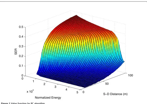
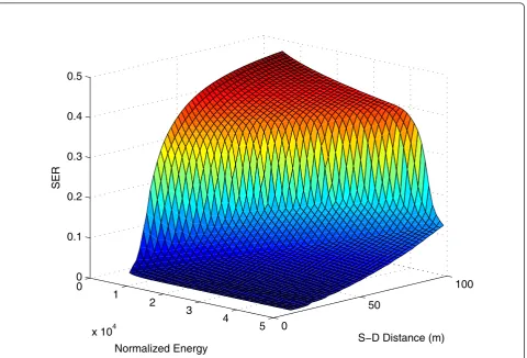
The first result is about the value function approxi-mating solution. The value function computed by using the RC method is plotted in Figure 1. For contrast, actual value function (i.e., the average energy consump-tion with respect to all states) obtained through simula-tion experiment is also presented in Figure 2. Two figures coincide very well. This demonstrates the cor-rectness of our theoretical analysis and derivation. The optimal value function can provide a precise prediction of the actual energy consumption in the networks.

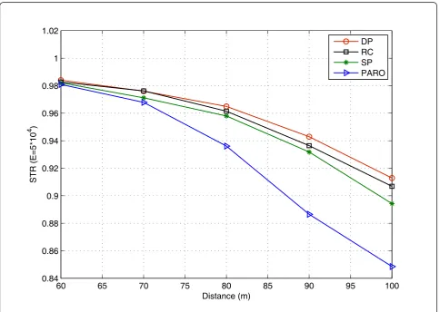
Figure 3 examines the SER performance in term of the source-to-end distance. It can be also observed that the proposed routing protocols by using DP and the RC algo-rithm outperform SP-power [19] and PARO algoalgo-rithms

[20]. Due to the pass loss effects, the SER values decreases when distance increases. At big distance values, it shows that the proposed protocol obtains much better performance. We can explain this as the following: our protocol takes into account the transmission power set-ting when making forwarding decision. Actually, by doing so, we add one more degree of freedom (i.e., the energy dimension) into the original routing problem. While traditional routing algorithms consider only the spatial dimension, our protocol exploits both energy and spatial dimensions. Thus, it has underly advantage over the traditional algorithms, which becomes much remark-able as the source-to-end distance increases. From Figure 3, it also shows that the optimal routing selection per-forms better than the RC, but the later is much simpler.

6. Conclusions

In this article, we have studied the joint optimization pro-blem of channel coding, resource allocation, and route planning for WSN using demodulation-and-forward pro-tocol at each relay node. The objective function is to find out the packet forwarding route with minimum FER sub-ject to the end-to-end energy consumption constraint.

0

1

2

3

4

5

x 104 0

50

100 0

0.1 0.2 0.3 0.4 0.5

S−D Distance (m) Normalized Energy

SER

Specifically, we cast this energy and QoS aware packet forwarding problem into the framework of dynamic pro-gramming. Then, a low-complexity, suboptimal approach is provided by performing the the route planing and power allocation separately. Simulation experiments are carried out to evaluate the performance of the proposed forwarding protocol. The results indicate that our proto-col significantly outperforms classical routing algorithms, and can achieve comparable performance with the opti-mal method.

Acknowledgements

This work was partially supported by the National Natural Science Foundation of China under Grant number 61071083.

Author details

1_{State Key Laboratory of Advanced Optical Communication Systems and}

Networks, School of Electronics Engineering and Computer Science, Peking University, Beijing, China2_{School of Electrical Engineering and Computer}

Science, Peking University, Beijing, China

Competing interests

The authors declare that they have no competing interests.

Received: 18 November 2011 Accepted: 29 March 2012 Published: 29 March 2012

References

1. IF Akyildiz, W Su, Y Sankarasubramaniam, E Cayirci, A survey on sensor networks. IEEE Commun Mag.40(8), 102_–114 (2002)

2. GJ Foschini, MJ Gans, On limits of wireless communications in a fading environment when using multiple antennas. Wirel Personal Commun.6, 311–335 (1998)

3. L Xiao, M Xiao, A new energy-efficient MIMO-sensor network architecture MSENMA, inVehicular Technology Conference 2004 Fall, Los Angeles, USA, (Sep 2004)

4. R Wang, M Tao, Joint source and relay precoding design for MIMO two-way relaying based on MSE criteria. IEEE Trans Signal Process.6(3), 1352_–1365 (2011)

5. S Cui, A Goldsmith, Energy-efficiency of MIMO and cooperative MIMO techniques in sensor networks. IEEE J Sel Areas Commun.22(6), 1089_–1098 (2004)

6. Y Liu, M Tao, Optimal channel and relay assignment in OFDM-based multi-relay multi-pair two-way communication networks. IEEE Trans Commun. 60(2), 317–321 (2012)

7. J Chen, W Xu, S He, Y Sun, P Thulasiramanz, X Shen, Utility-based asynchronous flow control algorithm for wireless sensor networks. IEEE J Sel Areas Commun.28(7), 1116–1126 (2010)

8. J Zhang, J Chen, Y Sun, Transmission power adjustment of wireless sensor networks using fuzzy control algorithm. Wirel Commun Mobile Computing (Wiley).9(6), 805–818 (2009)

9. B Zhang, H Mouftah, QoS routing for wireless ad hoc networks: problems, algorithms, and protocols. IEEE Commun Mag.43(10), 110–107 (2005) 10. B Zhang, H Mouftah, Z Zhao, J Ma, Localized power-aware alternate routing

for wireless ad hoc networks. Wirel Commun Mobile Comput.9(7), 882–893 (2009)

0 1

2 3

4 5

x 104 0

50

100 0

0.1 0.2 0.3 0.4 0.5

S−D Distance (m) Normalized Energy

SER

11. V Tarokh, N Seshadri, AR Calderbank, Space-time codes for high data rate wireless communication: performance criterion and code construction. IEEE Trans Inf Theory.44(2), 744–765 (1998)

12. L Song, Y Zhang, R Yu, W Yao, QoS-aware packet forwarding in MIMO sensor networks: a cross-layer approach. Wirel Commun Mobile Comput. 10(6) (2010)

13. Y Rong, Y Zhang, L Song, W Yao, oint Optimization of Power, Packet Forwarding and Reliability in MIMO Wireless Sensor Networks, ACM/ Springer Mobile Networks and Applications (MONET).16(10) (2010) 14. A Ephremides, Energy concerns in wireless networks. IEEE Wirel Commun.

9(4), 48–59 (2002)

15. JH Chang, L Tassiulas, Energy conserving routing in wireless ad-hoc networks, inProceedings of the Annual IEEE Conference on Computer

Communications, INFOCOM 2000, Tel-Aviv, Israel, pp. 22–31 (March 2000)

16. YT Hou, Y Shi, HD Sherali, SF Midkiff, On energy provisioning and relay node placement for wireless sensor networks. IEEE Trans Commun.4(5), 2579_–2590 (2005)

17. DP Bertsekas,Dynamic Programming and optimal control, (Athena Scientific, Belmont, MA, 1995)

18. MK Simon, MS Alouini,Digital Communications over Fading Channels: A Unified Approach to Performance Analysis, (Wiley Series in

Telecommunications and Signal Processing, USA, 2001)

19. I Stojmenovic, X Lin, Power-aware localized routing in wireless networks. IEEE Trans Parallel Dist Syst.12(11), 22_–33 (2001)

20. J Gomez, AT Campbell, M Naghshineh, C Bisdikian, PARO: Conserving transmission power in wireless ad hoc networks, inProc ICNP_’01, Mission Inn, Riverside, CA, pp. 24–34 (2001)

doi:10.1186/1687-1499-2012-125

Cite this article as:Wuet al.:QoS-aware multihop routing in wireless sensor networks with power control using demodulation-and-forward

protocol.EURASIP Journal on Wireless Communications and Networking

20122012:125.

Submit your manuscript to a

journal and benefi t from:

7 Convenient online submission

7 Rigorous peer review

7 Immediate publication on acceptance

7 Open access: articles freely available online

7 High visibility within the fi eld

7 Retaining the copyright to your article