R E S E A R C H
Open Access
Mathematical analysis and numerical
simulation of two-component system with
non-integer-order derivative in high
dimensions
Kolade M Owolabi
*and Abdon Atangana
*Correspondence: [email protected] Institute for Groundwater Studies, Faculty of Natural and Agricultural Sciences, University of the Free State, Bloemfontein, 9300, South Africa
Abstract
In this paper, we propose efficient and reliable numerical methods to solve two notable non-integer-order partial differential equations. The proposed algorithm adapts the Fourier spectral method in space, coupled with the exponential integrator scheme in time. As an advantage over existing methods, our method yields a full diagonal representation of the non-integer fractional operator, with better accuracy over a finite difference scheme. We realize in this work that evolution equations formulated in the form of fractional-in-space reaction-diffusion systems can result in some amazing examples of pattern formation. Numerical experiments are performed in two and three space dimensions to justify the theoretical results. Simulation results revealed that pattern formation in a fractional medium is practically the same as in classical reaction-diffusion scenarios.
MSC: 34A34; 35A05; 35K57; 65L05; 65M06; 93C10
Keywords: Fourier spectral method; exponential integrator; fractional reaction-diffusion; nonlinear PDEs; numerical simulations; Turing instability
1 Introduction
Systems with non-integer order are commonly referred to as fractional differential equa-tions. They are systems containing fractional integrals or fractional derivatives, which have received a lot of attention across disciplines such as biology, chemistry and physics. More importantly, they are mostly used in dynamical systems with chaotic and spatio-temporal dynamical behavior, quasi-chaotic dynamical systems, the dynamics of porous media or complex material and random walks with memory. The concepts of fractional differential equations, with fractional integral equations and fractional partial differential equations, have gained a wider application in diverse fields of applied science and engi-neering.
In some years back, the interest of some researchers was devoted to research on the equations involving the fractional differential equations applied to mechanics, physics, and other disciplines. For instance, the time-fractional reaction-diffusion equations have
been studied by Podlubny [], Podlubnyet al.[], Gorenfloet al.[], Guoet al.[],
Aguilaret al.[–], Zhou [], Ilicet al.[] and Kilbaset al.[] and the references therein, to mention a few. The interested reader is referred to the monographs and literature on fractional calculus.
However, recent years have been characterized by fast growing applications of fractional calculus to various scientific and engineering fields pertaining to anomalous diffusion, signal processing and control, constitutive modelling in viscoelasticity, image processing, fluid mechanics and findings on soft matter behavior, to mention a few. Unlike the integer-order ordinary or partial differential equations, fractional calculus is capable of providing a more detail, simple and accurate description of complex dynamical, mechanical, chemical and physical processes that feature historical dependence and space non-locality, which has induced the occurrences of a series of fractional differential equations.
However, the mathematical theory and the efficient numerical algorithms of fractional-order differential equations require further study. Most analytical solutions obtained for fractional differential problems are given in terms of special functions, which make numer-ical evaluation difficult and almost impossible. Until now, finite difference schemes and series approximation techniques such as the variational iteration method and the Ado-mian decomposition method remain the dominant numerical methods for the solution of fractional reaction-diffusion equations.
More importantly, little is now known about the systematic analyses on the issue of sta-bility of numerical methods regarding fractional calculus, together with the solution tech-niques for high-dimensional fractional reaction-diffusion equations, most especially for nonlinear equations. The present paper introduces the Fourier spectral method as a better alternative to finite difference methods for solving fractional-in-space reaction-diffusion systems in one and high dimensions.
The remainder part of this paper is broken into sections. In Section , we introduce the general two-components partial differential equations formulated in both classical and fractional reaction-diffusion systems. We provide conditions for the emergence of Turing instability in the two scenarios. Section deals with the basics of fractional derivatives and various methods of numerical approximations. Numerical experiments in high dimen-sions are presented with some notable examples taken from the literature in Section . Section concludes the paper.
2 Model equation
In this section, we consider a two species scaled and nondimensionalized system in the form [–]
∂u(x,t) ∂t =Du
u(x,t) +F(u,v), ∂v(x,t)
∂t =Dvv(x,t) +G(u,v),
(.)
whereu(x,t),v(x,t) are used to describe the concentration of species at spatial positionx
and timet, due to the presence od diffusion, with respective diffusion coefficientsDu>
,Dv> . The nonlinear functions describing the reaction kinetics are given byFandG.
System (.) can be solved using any of the boundary conditions, namely Neumann
(zero-flux), Dirichlet, periodic or Robin type on bounded domain⊂Rn. The chemical species
concentrations are specified att= ,∀x∈.
subject to zero-flux boundary conditionsνuv= , on∂×[,T) with the initial function
u=uv=von× {t= }, on smooth and bounded domain, satisfying the conditions:
(i) existence and uniqueness, (ii) existence for all timest, (iii) continuously dependency on
the initial functions, (iv) for non-negative initial data, the solution is non-negative, and (v) the solution is bounded for all given bounded initial data.
Definition .(Sectorial operator []) Let operatorAbe linear in a Banach space,
de-noted B, and assumeAis dense and closely defined. If there exista,ω∈(,π),M≥,
such that
ρ(A)⊃=λ∈C|ϕ≤arg(λ–a)≤π,λ=a
and
Rλ(A)≤ M
|λ–a| for allλ∈
, (.)
whereAis defined as a sectorial operator.
Theorem . If A is given as a sectorial operator,then–A is the corresponding infinites-imal generator of an analytic semigroup,G(t).IfReλ>a,a∈R,wheneverλ∈σ(A)then,
for any t> ,
G(t)≤Cexp(–at), AG(t)≤C
t exp(–at).
Hence,
d
dtG(t) = –AG(t), t> .
Proof The reader is referred to Theorem .. in [].
Lemma . If u and v are continuous from[,T]to Lp(),then the integrals
I(t) = t
G(t–τ)Fτ,u(τ),v(τ)dτ,
I(t) = t
G(t–τ)Gτ,u(τ),v(τ)dτ,
exist,Gand Gare the respective analytical semigroup of the Laplacian operatorsL= – and D(L),Iand Iare continuous on[,T)with I(t),I(t)∈D(L)and I(t),I(t)→+in Lpfor t→+.
Proof If the reaction-diffusion system (.) has a classical solution, thenuandvsatisfy
u(t) =G(t)u+
t
G(t–τ)F(τ,u(τ),v(τ))dτ, v(t) =G(t)v+tG(t–τ)G(τ,u(τ),v(τ))dτ.
The continuity ofu,vindicates continuity oft→F(u(t),v(t),t) andt→G(u(t),v(t),t),
so that the linear problems∂tU–U=F(u(t),v(t),t) and ∂tV–DV =G(u(t),v(t),t)
andU() =u,V() =vhave a unique solution. For details of the proof, see Lemma ..
in [].
Theorem .(Local existence [, ]) Assume the following conditions.
(c) D> ;
are satisfied.Then there exists T =T(u,v)such that the reaction-diffusion system(.)
possesses a unique solution(u,v)∈[CL∞((,T];D(Hα))]with u() =u∈CL∞and v() =
v∈CL∞.Forα≥we give the fractional powers of the Helmholtz operatorH= –+I,
which we denoteHandD(Hα)as the domain of fractional powers ofH.
Proof It suffices to establish the corresponding result for (.). See a similar proof in [],
Theorem .., which utilized Banach’s fixed point theorem for establishing the result.
2.1 Classical two-components reaction-diffusion systems
A Turing instability (diffusion-driven instability) arises when a homogeneous steady state solution of the reaction system of the form (.) is linearly stable to some perturbations
in the absence of the diffusion terms (Du,Dv) but linearly unstable in the presence of
dif-fusion to small spatial perturbations. A spatially uniform steady state of the system (.)
is the state (u∗,v∗) :F(u∗,v∗) =G(u∗,v∗) = in such a way thatu=u∗,v=v∗satisfies the
boundary conditions. For instance, using a zero-flux boundary condition on a rectangular domain, for diffusion-driven instability to occur, the conditions
∂F
must be satisfied. We evaluate the partial derivatives ofFandGat the stationary uniform
state (u∗,v∗), that is, the zeros ofFandG. The linear stability for the time evolution of the
perturbations
∇u(x,t),∇v(x,t)
about the equilibrium steady state (u∗,v∗) in the standard two-components system are
where D=Du/Dv denotes the diffusivity ratio,λ> is a scaling variable which can be defined as the relative strength of the reaction kinetics or as the linear size of the spatial domain, and
ai,j=
∂Fi
∂nj
,∂Gi
∂nj
.
Next, for simplicity, we adopt the Laplace transform technique in the case of anomalous diffusion to find the Turing conditions. On applying a temporal Laplace and spatial Fourier transform, we obtain
u(k,r) =(r+Dk
–λa)u(k,t= ) +λav(k,t= )
(r+k–λa)(r+Dk–λa) –λaa ,
v(k,r) = (r+k
–λa
)v(k,t= ) +λu(k,t= )
(r+k–λa)(r+Dk–λa) –λaa ,
wherek,rare the Fourier and Laplace transform variables, the tilde and hat symbols
de-note, respectively, the Fourier and Laplace transformed variables. By finding the inverse of the Laplace transforms, we obtain the perturbations temporal growth
r+k–λar+Dk–λa–λaa=r–s(k)r–s(k) (.) after factorizing the denominator and using partial fractions. If the roots in (.) are found to be distinct, the inverted canonical expression can be written in the form
z(k,r) =
j=
β–j(k)
r–sj(k) ,
with the corresponding inverse Laplace transform as
z(k,t) =
j=
β–j(k)esj(k)t.
For any of the roots to be positive (that is, having a real component greater than zero), the homogeneous steady state becomes linearly unstable, but linearly stable if otherwise. In what follows, we quickly summarized the conditions for a Turing (diffusion-driven)
instability as (i)(s(k= )) < ,(s(k= )) < , and (ii)(s(k> )) > ,(s(k> )) > ,
withsqdefined as the zeros of the quadratic equation
p(s) =s+k–λas+Dk–λa–λaa.
It follows from equation (.) that, with the conditionsa+a< andaaaa> ,
condition (i) is consistent, but not so for (ii) in conjunction with (i) ifD= . Conditions (i)
and (ii) cannot be attained simultaneously ifD≤. In the physical sense, it implies that
2.2 General two-components fractional reaction-diffusion systems
So far, we have examined the classical reaction-diffusion system. Here, we now consider the fraction reaction-diffusion system, a special case of (.) written in the general form
∂u(x,t)
where <α≤ is termed the fractional power or mostly regarded as the anomalous
diffu-sion exponent of the species’u(x,t),v(x,t) concentrations. The parameterλand functions
FandGremain as earlier defined, and as illustrated in [–], we have
αu(x,t) = ∂
with a similar expression for v, is the generalization of the diffusion operator from
standard to fractional. When solving the system with the Laplace transform, the term
L–{∂α–
∂tα–∇u(x,t)|t=}actually preludes the introduction of nonphysical terms.
Proceed-ing as earlier mentioned, a perturbation about point (u∗,v∗) results in the linearized
equa-tions
By adopting the techniques of spatial Fourier and temporal Laplace transforms, we get
ru(k,r) –u˜(k,t= ) =λau(k,r) +av(k,r)
–rαku(k,r),
rv(k,r) –v˜(k,t= ) =λau(k,r) +au(k,r)–rαkv(k,r),
which we decouple as
Thus, we obtain the conditions for the diffusion-driven case in the fractional reaction-diffusion system by finding the inverse of the Laplace transforms. So in this work, we
classified the scaling of the fractional powerαinto subdiffusion when <α< [, ],
advection flow equation whenα= [, ], and superdiffusion when <α< [, ]. In
numerical experiments, our results will be based on these classifications.
3 Fractional derivatives and adaptive numerical approaches
By replacing Fick’s law for the flux U (which governs the rate at which mass is trans-ported through an unit area against the concentration gradient) by its fractional derivative, a space-fractional diffusion equation can be derived in the form []
with the initial function
ui(x, ) =ui(x), i= , , . . . ,n, (.)
subject to any of the boundary conditions:
• In the case of an infinite system,x∈(–∞,∞), hereRis a subset of(–∞,∞).
• x∈[,L],∂∂uix(,t) =∂∂uix(L,t) = ,i= , , . . . ,n, no-flux or Neumann boundary
condition for a finite system.
• x∈[,L], u(,t) = u(L,t) = ua,i= , , . . . ,n, called the Dirichlet or fixed concentration
boundary condition, also for a fixed system.
Hereui(t, x)∈Rn,Fi: Rn→RandDis the diffusion tensor, andα= (∂ the Riemann-Liouville fractional gradient, for
∂α
∂zα having similar expressions.
3.1 Integral representation of fractional derivative
In what follows, we shall describe the most two popular integral representation of frac-tional derivative via the Caputo and Riesz integral representations of the diffusion equa-tion.
.. Caputo space-fractional derivative
A space-fractional diffusion equation takes the form
∂u
aDαx defines the fractional derivative in the Caputo sense [, ]
By mimicking the approach suggested in [, ], we can recast the fractional-in-space diffusion equation (.) to become an ODE,
dul
.. Riesz space-fractional derivative
In a similar fashion, a space-fractional diffusion equation can be taken as
∂u
xis the Riesz fractional derivative, with expression
R
In this sense,xI±–αis used to represent the Riemann-Liouville (or Weyl) fractional integrals,
defined as
and, recovering the Riesz potential, we have
xI–αu(x) =
In the interval <α< , which corresponds to the superdiffusive scenario, we define the
In the spirit of Liuet al.[, ], we have the following equivalent ODE for (.):
Many others integral representations of the fractional derivatives are well classified in [, , , –, , ].
3.2 Numerical techniques for fractional diffusion equation
In this section, we do not intend to go into details, but we report a brief survey of some of the numerical approaches that have been used. Several numerical techniques have been used in the literature to circumvent the non-local restrictions associated with the space-fractional operators. Some of these methods include finite element, finite difference and spectral methods, to mention a few.
.. Finite difference method
Over the years, many time dependent partial differential equations have combined low-order nonlinear with higher-low-order linear terms. Until now, numerical simulation of most physical models still relied on a low-order finite difference scheme to discretize both the space- and time-fractional-order derivatives, which are largely encountered in the fields of computational physics and mathematics. While the finite difference scheme remains simple, straightforward and easy-to-code for the integration of integer-order (classical) differential equations, its applicability is reduced for fractional-order differential equations as it results to systems of linear equation defined by dense or large full matrices.
A finite difference (FD) discretization of the fractional-order differential equation can be obtained by using the well-known shifted Grünwald-Letnikov approximation of the Riemann-Liouville derivatives [, , ]. Here, we provide a further approximation by applying the FD method to solving the space-fractional diffusion equation
∂u
applications. The scenario of non-integer <α< is used to model the superdiffusive
case in which a cloud of particles spreads at a faster rate than in the classical diffusion
model. It should be noted that we have the classical advective flow equation whenα=
and standard diffusion equation wheneverα= .
By using the FD method to approximate space derivatives first in the classical medium
α= , equation (.) can be written in the matrix form
du
whereδ=D/hand
.. Finite element method
With the finite element method, the exact solution is usually approximated with expansion
in terms of piecewise polynomialsφj(x):
u(x,t)≈ N
j=
uj(t)φj(x).
The basis functionφj(x) has a compact support which corresponds to the nodejof a mesh
(or grid) that divides the computational domain inN– segments with step-lengthh=
L/(N– ). The position of nodejis denotedxj, and computing the fractional derivative
of the solution then amounts to computing the fractional derivative of all basis functions
φj(x); see Hanert [, ] for details.
the dense matrix structure; to get optimal convergence would tremendously amount to an increase in the radius of truncation [, ].
.. Fourier spectral method
A little attention has been given to spectral method despite its desired ability to achieve higher-order convergence (accuracy and efficiency) over the existing low-order schemes such as finite difference and finite element schemes when applied to solve fractional-in-space reaction-diffusion equations. Application of spectral methods for the solution of classical reaction-diffusion problems is considered to be relatively simple and, being a sub-ject of mathematical and theoretical studies for some years, has been by now examined almost completely. However, the case of fractional-order reaction-diffusion is still poorly understood with just a handful of papers addressing the problems with spectral methods. Some of the little work done on spectral methods is [, –].
For spectral representation, we letH be the real Hilbert space inL(,L), and
con-sider the operator T : H→ H defined by Tϕ =ϕ = dxdϕ on H ={ϕ ∈ H;ϕ,ϕ ∈
L(,L) are continuous with boundary conditionB(ϕ) = }. ThenTϕn=λnϕn,n= , , . . . .
For anyϕ∈H,
ϕ=
∞
n=
cnϕn, cn=ϕ,ϕn and Tϕ=
∞
n= λncnϕn.
So, if is a continuous function onR, then
(T)ϕ=
∞
n=
(λn)cnϕn, (.)
provided ∞n=|(λn)cn|,∞.
For the space discretization, we consider the one-dimensional fractional-in-space
dif-fusion equation (.) above, subject to initial conditionu(x, ) =u(x) and homogeneous
boundary conditions clamped at the extreme ends of spatial domainx∈[a,b]. By relating
(.) with the technique in [], the fractional Laplacian ()αcan be defined in the space
of functions
Hα () =
u=
∞
j=
ajλα∈L() :uHα()=
!∞
j= ajλα
"/
<∞
, (.)
where
uHα()=()αuL(). (.)
Therefore for anyu∈Hα
, the Laplacian ()αis defined by
αu=
∞
i=
ajλαjϕj, (.)
For homogeneous Dirichlet boundary condition we obtain
and for homogeneous Neumann boundary condition we get
(ϕj,λj) =
Next, we want to extend this approach to higher-dimensional two-component fractional-in-space reaction-diffusion system (.) in the presence of reaction (source) terms; by applying the fast Fourier transform we obtain
Ut(ωx,ωy,t) =δ
integrating factors, by setting
U=eδαtU¯, V=eδαtV¯,
At this point, we can now discretize the square domain on equi-spaced number of points
NxandNyin the spatial directionsxandy. We adapt the discrete fast Fourier transform
(DFFT) [] to transform (.) to a system of ODEs
∂tU¯i,j=eKu
order time integration methods can be naturally used in conjunction with high resolu-tion spectral methods to obtain efficient and accurate approximaresolu-tions of the phase field models.
.. Time stepping method
For the temporal discretization, we employ the modified Krogstad [, ] version of the exponential time differencing Runge-Kutta method that was earlier proposed by Cox and Matthews []. It reads
Wn+=eLdtWn+γN(Wn,tn) +γ
whereW=W(u,v), L, N defined as linear and nonlinear operators with variable
coeffi-cients
To overcome the pronounced cancelation errors associated with the higher-order expo-nential time differencing Runge-Kutta method, the three coefficients in (.) suffer se-rious cancelation errors when the eigenvalues of L are close to zero. The vulnerability cancelation errors in the higher-order variants can render the whole schemes useless. As a result, modified exponential time differencing (ETD) schemes are proposed by using the complex contour integrals
f(L) =
πi
f(t)(tI– L)–dt
here is the contour that encloses the eigenvalues ofl []. Details of derivation and
stability analysis of scheme (.), which we denote for brevity in this paper ETDRK, can be found in [, , –]. In the past, ETD schemes have also been used by some authors under different names [–].
.. Convergence analysis
of the schemes by reporting the error norm∞in the numerical experiment att= as
whereu˜ anduare the respective approximate and exact solutions, andNis the number
of computational grids.
By using (. and (.), a straightforward analytical solution of (.) can be presented as
boundary conditions (.) and (.). Fourier spectral methods denote the truncated se-ries expansion of (.) when a finite number of orthonormal trigonometric
eigenfunc-tions{ϕj}are considered, that is,
For the space convergence, the solution of diffusion equation (.) using a finite difference or finite element matrix-based technique can be approximated by
u(t)≈Ldiagexp–Dλαt,exp–Dλαt, . . . ,exp–DλαN–tL–u, (.)
where L denotes the corresponding eigenvectors matrix, and u represents the vector node
ofu[, ]. Obviously, both (.) and (.) are exact in time, to study the convergence
of the two schemes used for numerical approximation of (.) we proceed by using a simple example. Hence, we consider for simplicity a one-dimensional fractional-in-space diffu-sion benchmark problem with simple source term [, , ], which consists of finding
u(x,t) such that
Convergence results for finite differences and Fourier spectral methods are at varyingα
are displayed in Figure (a–b), respectively. Also in Figure , we present the numerical
results justifying the performance of both finite difference and Fourier spectral methods
at some instances ofα. Panel (c) shows the comparison between the exact (solid-lines) and
Figure 1 Solution of fractional-in-space diffusion equation (3.24) showing the trade-off between finite difference and Fourier spectral methods at different instances ofαand simulation timet, for
D= 10.
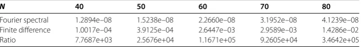
Table 1 The relative error for fractional diffusion equation for various values of discretization, atD= 0.25 andt= 5
N 40 50 60 70 80
Fourier spectral 1.2894e–08 1.5238e–08 2.2660e–08 3.1952e–08 4.1239e–08 Finite difference 1.0017e–04 3.9125e–04 2.6447e–03 2.9589e–03 1.4286e–02
Ratio 7.7687e+03 2.5676e+04 1.1671e+05 9.2605e+04 3.4642e+05
is obtained at different instances of timet= (, , , ) at fractional valueα= ..
Com-parison in panels (a) and (b) fort= and the relative error results in Table justify well
enough abandoning the finite difference method in the remaining part of this work.
4 Numerical experiments
In this section, we illustrate the mathematical techniques presented in the previous sec-tions with some numerical examples in one, two, and probably three dimensions. We first consider the fractional-in-space reaction-diffusion system (.) and focus on the re-scaled Beddington-DeAngelis functional response with logistic growth term [–],
F(u,v) =σu( –u)(β+u+v) –uv, G(u,v) =γuv–δv(β+u+v). (.)
In order to give a good working guideline on the appropriate choice of parameters when numerically simulating the full fractional reaction-diffusion system, it is necessary to
G(u,v) = , it is not difficult to see that model (.) with kinetics (.) possesses three
equi-librium points in the absence of diffusion. The first point when (u∗,v∗) = (, ) corresponds
to total washout of both populations, while (u∗,v∗) = (, ) or vise versa corresponds to
ex-istence of one population. The third equilibrium point
u∗,v∗=
σ γ–γ+δ+&(σ γ–γ+δ)+ σ γ δβ
σ γ ,
γ δ –
u∗–β
is a trivial state which corresponds to the coexistence of both prey and predator. It is the
dynamics in the biologically meaningful regionu≥,v≥ which is of great interest.
The Jacobian or community matrix that corresponds to the interior equilibrium point
(u∗,v∗) is given by
J=
!
a a a a
"
=
!
σAB–σu∗B+σu∗A–v∗ σu∗A–u∗ γv∗–δv∗ γu∗–δB–δv∗,
"
(.)
whereA= (–u∗) andB= (β+u∗+v∗). To ensure that the point (u∗,v∗) satisfies|J(u∗,v∗)|>
, it is necessary to keepβ in the interval (,γ–δδ ) when numerically simulating the full
system.
For the second example, we shall focus on the specific type II functional response [],
F(u,v) =u( –u) – uv
u+σ, G(u,v) = βuv
u+σ –γv. (.)
The equilibrium point (u∗,v∗) corresponding to the existence of both species is given by
u∗= σ γ
β–γ, v
∗= –u∗u∗+σ, β>γ andσ<β–γ γ .
Details of the linear stability analysis of kinetics (.) can be found in [, ].
It is clear from the results obtained in Figure that the two species oscillate in phase. The populations profile in (a) which correspond to the coexistence of the species are unstable with initial time but become stable as time is increasing. It is otherwise with kinetics (.) in plot (c), where the species are stable with initial time and become unstable with
spatio-temporal oscillations at bigger time, sayt= ,.
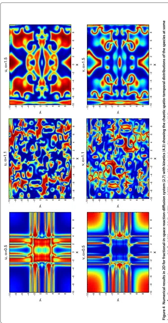
4.1 Two-dimensional results
In order to give a better illustration of the theoretical results and some biological wave phe-nomena of the fractional-in-space system describing spatial predator-prey interactions, we present in this subsection some numerical results in two space dimensions (D). We
letx,y∈R,α= (∂α/∂xα+∂α/∂yα) and experiment on a growing domain in the interval
[–L,L] subject to Neumann boundary conditions clamped at the domain extreme ends,
and initial conditions specifically chosen as
u(x,y, ) = –exp–(x– /)+ (y– /),
v(x,y, ) =exp–(x– /)+ (y– /),
(.)
Figure 2 Time series and limit cycles for system (2.7) with kinetics (4.1) [upper row] and (4.3) [lower row], respectively.Parameter values:(a),(b)σ= 0.5,β= 0.032,γ= 0.8,δ= 0.3 andt= 4,000. For panels (c),(d)σ= 0.25,β= 1.05,γ= 0.5 att= 100 and initial data (u0,v0) = (0.25, 0.15).
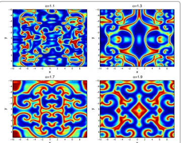
In the experiment with kinetics (.), it was found that the two species have similar
pattern distributions. As a result, we report only that of speciesuas shown in Figure .
The effects of fractional powerαare shown to be more pronounced in the subdiffusive
case whenα= . and superdiffusive scenario atα= .. The unsteady oscillatory patterns
indicate the presence of a Turing instability. The evolution of more complex spiral patterns
is shown in Figure for kinetics (.) at different instances of fractional indexα at time
t= ,. The upper and lower rows represents the distribution patterns of speciesuand
v, respectively, with varying values ofα. We further report some complex spiral patterns
distribution for vin Figure in the fractional regime <α< , which we classify as a
superdiffusive case. It should be mentioned that other Turing patterns can be observed, depending on the choice of initial and parameter values.
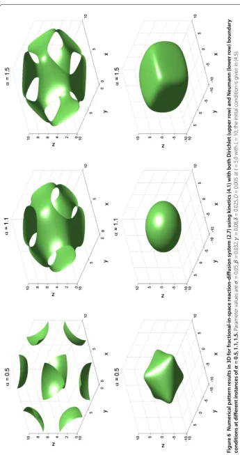
4.2 Three-dimensional results
In the spirit of [–], we further explore some of the dynamic richness of fractional-in-space reaction-diffusion, we extend our numerical experiments to three fractional-in-space dimensions
(D). As usual, we letx,y,z∈R,α= (∂α/∂xα+∂α/∂yα+∂α/∂zα) denote the Laplacian
op-erator with fractional orderα. As discussed in Section , our numerical simulation results
apply to general boundary conditions, but for the sake of ease of exposition we first
exper-iment on a growing domain of size [–L,L] subject to Neumann boundary conditions and
Figure 5 Evolution of spatio-temporal complex spiral patterns ofvfor kinetics (4.3) at superdiffusive scenarios.Parameter values and initial data as in Figure 4.
condition. For both kinetics, we focus on the initial functions
u(x,y,z, ) = – .exp–(x–s/)+ (y–s/)+ (z–s/),
v(x,y,z, ) = .exp–(x–s/)+ (y–s/)+ (z–s/), s= .
(.)
In Figure , we observed different amazing patterns for the distributions of speciesv. We
considered two important boundary conditions to explore the variability in D patterns for the fractional-in-space reaction-diffusion system. We should also inform the reader that other pattern scenarios are possible and subject to the choice of initial functions, boundary conditions, fractional power index value and the domain size.
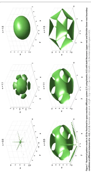
Similarly in Figure , we experiment with system (.) with kinetics (.). It was also
found that the distributions of speciesuandvare almost of the same type. As a result,
we present the evolutions of speciesuin D with both Neumann and Dirichlet boundary
conditions as shown in the upper and lower rows, respectively. Other patterns are possible depending on the choice of parameters and initial conditions.
5 Conclusion
cretization, we employ a fractional exponential integrator whose formulation is based on fourth order exponential time differencing to advance the resulting coupled system of or-dinary differential equations in time. Two notable examples of reaction-diffusion systems taken from the literature are considered and formulated in space-fractional form. Our sim-ulation results for the chosen examples show that pattern formations in the subdiffusive
( <α< ) and superdiffisive ( <α< ) scenarios are practically the same case as with the
standard reaction-diffusion problems. The dynamic richness of our numerical techniques is explored in two and three space dimensions. The methodology in this research can be extended to solve multi-components integer- and non-integer-order systems.
Competing interests
The authors declare that there is no conflict of interests regarding the publication of this paper.
Authors’ contributions
All authors read and approved the final manuscript.
Publisher’s Note
Springer Nature remains neutral with regard to jurisdictional claims in published maps and institutional affiliations.
Received: 6 April 2017 Accepted: 19 July 2017
References
1. Podlubny, I: Fractional Differential Equations. Academic Press, San Diego (1999)
2. Podlubny, I, Chechkin, A, Skovranek, T, Chen, YQ, Jara, BB: Matrix approach to discrete fractional calculus II: partial fractional differential equations. J. Comput. Phys.228, 3137-3153 (2009)
3. Gorenrenflo, R, Luchko, Y, Mainardi, F: Wright function as scale-invariant solutions of the diffusion-wave equation. J. Comput. Appl. Math.118, 175-191 (2000)
4. Guo, B, Pu, X, Huang, F: Fractional Partial Differential Equations and Their Numerical Solutions. World Scientific, Singapore (2011)
5. Gómex-Aguilar, JF, López-López, MG, Alvarando-Martínez, VM, Reyes-Reyes, J, Adam-Medina, M: Modeling diffusive transport with a fractional derivative without singular kernel. Phys. A, Stat. Mech. Appl.447, 467-481 (2016) 6. Gómez-Aguilar, JF, Escobar-Jiménez, RF, Olivares-Peregrino, VH, Benavides-Cruz, M, Calderón-Ramón, C: Nonlocal
electrical diffusion equation. Int. J. Mod. Phys. C27, 1650007 (2016)
7. Gómex-Aguilar, JF, Miranda-Hernández, M, López-López, MG, Alvarando-Martínez, VM, Baleanu, D: Modeling and simulation of the fractional space-time diffusion equation. Commun. Nonlinear Sci. Numer. Simul.30, 115-127 (2016) 8. Gómez-Aguilar, JF: Space-time fractional diffusion equation using a derivative with nonsingular and regular kernel.
Phys. A, Stat. Mech. Appl.465, 562-572 (2017)
9. Zhou, Y: Basic Theory of Fractional Differential Equations. World Scientific, New Jersey (2014)
10. Ilic, M, Liu, F, Turner, I, Anh, V: Numerical approximation of fractional-in-space diffusion equation, I. Fract. Calc. Appl. Anal.8, 323-341 (2005)
11. Kilbas, AA, Srivastava, HM, Trujillo, JJ: Theory and Applications of Fractional Differential Equations. Elsevier, New York (2006)
12. Murray, JD: Mathematical Biology II: Spatial Models and Biomedical Applications. Springer, Berlin (2003) 13. Owolabi, KM, Patidar, KC: Numerical simulations of multicomponent ecological models with adaptive methods.
Theor. Biol. Med. Model.13, 1 (2016). doi:10.1186/s12976-016-0027-4
14. Owolabi, KM: Mathematical analysis and numerical simulation of patterns in fractional and classical reaction-diffusion systems. Chaos Solitons Fractals93, 89-98 (2016)
15. Henry, D: Geometric Theory of Semilinear Parabolic Equations. Springer, Berlin (1981)
16. Hollis, SL, Martin, RH, Pierre, M: Global existence and boundedness in reaction-diffusion systems. SIAM J. Math. Anal.
18, 744-761 (1987)
17. Henry, BI, Wearne, SL: Fractional reaction-diffusion. Physica A276, 448-455 (2000)
18. Henry, BI, Wearne, SL: Existence of Turing instabilities in a two-species fractional reaction-diffusion system. SIAM J. Appl. Math.62, 870-887 (2002)
19. Pindza, E, Owolabi, KM: Fourier spectral method for higher order space fractional reaction-diffusion equations. Commun. Nonlinear Sci. Numer. Simul.40, 112-128 (2016). doi:10.1016/j.cnsns.2016.04.020
20. Zeng, F, Li, C, Liu, F, Turner, I: Numerical algorithms for time-fractional subdiffusion equation with second-order accuracy. SIAM J. Sci. Comput.37, A55-A78 (2015)
21. Zheng, M, Liu, F, Turner, I, Anh, V: A novel high order space-time spectral method for the time fractional Fokker-Planck equation. SIAM J. Sci. Comput.37, A701-A724 (2015)
22. Zeng, F, Liu, F, Li, C, Burrage, K, Turner, I, Anh, V: A Crank-Nicolson ADI spectral method for a two-dimensional Riesz space fractional nonlinear reaction-diffusion equation. SIAM J. Numer. Anal.52, 2599-2622 (2014)
23. Meerschaert, MM, Mortensenb, J, Wheatcraft, SW: Fractional vector calculus for fractional advection-dispersion. Physica A367, 181-190 (2006)
25. Liu, F, Anh, V, Turner, I, Zhuang, P: Numerical simulation for solute transport in fractal porous media. ANZIAM J.45, 461-473 (2004)
26. Ortigueira, MD: Fractional Calculus for Scientists and Engineers. Springer, New York (2011)
27. Atangana, A: On the stability and convergence of the time-fractional variable order telegraph equation. J. Comput. Phys.293, 104-114 (2015)
28. Meerschaert, MM, Tadjeran, C: Finite difference approximations for two-sided space-fractional partial differential equations. Appl. Numer. Math.56, 80-90 (2006)
29. Hanert, E: A comparison of three Eulerian numerical methods for fractional-order transport models. Environ. Fluid Mech.10, 7-20 (2010). doi:10.1007/s10652-009-9145-4
30. Hanert, E: On the numerical solution of space-time fractional diffusion models. Comput. Fluids46, 33-39 (2011). doi:10.1016/j.compfluid.2010.08.010
31. Roop, J: Computational aspects of FEM approximations of fractional advection dispersion equations on bounded domains onR2. J. Comput. Appl. Math.193, 243-268 (2005)
32. Bueno-Orovio, A, Kay, D, Burrage, K: Fourier spectral methods for fractional-in-space reaction-diffusion equations. BIT Numer. Math.54, 937-954 (2014)
33. Khader, MM: On the numerical solutions for the fractional diffusion equation. Commun. Nonlinear Sci. Numer. Simul.
16, 2535-2542 (2010)
34. Li, X, Xu, C: Existence and uniqueness of the weak solution of the space-time fractional diffusion equation and a spectral method approximation. Commun. Comput. Phys.8, 1016-1051 (2010)
35. Owolabi, KM, Patidar, KC: Existence and permanence in a diffusive KiSS model with robust numerical simulations. Int. J. Differ. Equ.2015, 485860 (2015). doi:10.1155/2015/485860
36. Krogstad, S: Generalized integrating factor methods for stiff PDEs. J. Comput. Phys.203, 72-88 (2005) 37. Owolabi, KM: Numerical solution of diffusive HBV model in a fractional medium. SpringerPlus5, 1643 (2016).
doi:10.1186/s40064-016-3295-x
38. Cox, SM, Matthews, PC: Exponential time differencing for stiff systems. J. Comput. Phys.176, 430-455 (2002) 39. Kassam, AK, Trefethen, LN: Fourth-order time stepping for stiff PDEs. SIAM J. Sci. Comput.26, 1214-1233 (2005) 40. Du, Q, Zhu, W: Analysis and applications of the exponential time differencing schemes and their contour integration
modifications. BIT Numer. Math.45, 307-328 (2005)
41. Owolabi, KM, Patidar, KC: Higher-order time-stepping methods for time-dependent reaction-diffusion equations arising in biology. Appl. Math. Comput.240, 30-50 (2014). doi:10.1016/j.amc.2014.04.055
42. Owolabi, KM, Patidar, KC: Numerical solution of singular patterns in one-dimensional Gray-Scott-like models. Int. J. Nonlinear Sci. Numer. Simul.15, 437-462 (2014). doi:10.1515/ijnsns-2013-0124
43. Owolabi, KM, Patidar, KC: Effect of spatial configuration of an extended nonlinear Kierstead-Slobodkin reaction-transport model with adaptive numerical scheme. SpringerPlus5, 303 (2016).
doi:10.1186/s40064-016-1941-y
44. Beylkin, G, Keiser, JM, Vozovoi, L: A new class of time discretization schemes for the solution of nonlinear PDEs. J. Comput. Phys.147, 362-387 (1998)
45. Du, Q, Zhu, W: Stability analysis and applications of the exponential time differencing schemes. J. Comput. Math.22, 200-209 (2004)
46. Mott, DR, Oran, ES, van Leer, B: A quasi-steady-state solver for the stiff ordinary differential equations of reaction kinetics. J. Comput. Phys.164, 407-468 (2002)
47. Yang, Q, Turner, I, Liu, F, Ili´c, M: Novel numerical methods for solving the time-space fractional diffusion equation in 2D. SIAM J. Sci. Comput.33, 1159-1180 (2011)
48. Guo, HJ, Chen, XX: Existence and global attractivity of positive periodic solution for a Volterra model with mutual interference and Beddington-DeAngelis functional response. Appl. Math. Comput.217, 5830-5837 (2011) 49. Haque, M: A detailed study of the Beddington-DeAngelis predator-prey model. Math. Biosci.234, 1-16 (2011) 50. Li, HY, Takeuchi, Y: Dynamics of the density dependent predator-prey system with Beddington-DeAngelis functional
response. J. Math. Anal. Appl.374, 644-654 (2011)
51. Xue, L: Pattern formation in a predator-prey model with spatial effect. Physica A391, 5987-5996 (2012) 52. Garvie, M: Finite-difference schemes for reaction-diffusion equations modeling predator-pray interactions in
MATLAB. Bull. Math. Biol.69, 931-956 (2007)
53. Garvie, M, Trenchea, C: Spatiotemporal dynamics of two generic predator-prey models. J. Biol. Dyn.4, 559-570 (2010) 54. Owolabi, KM: Robust and adaptive techniques for numerical simulation of nonlinear partial differential equations of
fractional order. Commun. Nonlinear Sci. Numer. Simul.44, 304-317 (2016). doi:10.1016/j.cnsns.2016.04.021 55. Owolabi, KM, Atangana, A: Numerical solution of fractional-in-space nonlinear Schrodinger equation with the Riesz
fractional derivative. Eur. Phys. J. Plus131, 335 (2016). doi:10.1140/epjp/i2016-16335-8
![Figure 2 Time series and limit cycles for system (2.7) with kinetics (4.1) [upper row] and (4.3) [lower](https://thumb-us.123doks.com/thumbv2/123dok_us/961562.1117888/17.595.116.479.81.368/figure-time-series-limit-cycles-kinetics-upper-lower.webp)