R E S E A R C H A R T I C L E
Open Access
Numerical solution of linear integral
equations system using the Bernstein
collocation method
Ahmad Jafarian
1, Safa A Measoomy Nia
1, Alireza K Golmankhaneh
2and Dumitru Baleanu
3,4,5**Correspondence:
3Department of Mathematics and
Computer Sciences, Faculty of Art and Sciences, Çankaya University, Balgat, Ankara, 0630, Turkey
4Department of Chemical and
Materials Engineering, Faculty of Engineering, King Abdulaziz University, P.O. Box 80204, Jeddah, 21589, Saudi Arabia
Full list of author information is available at the end of the article
Abstract
Since in some application mathematical problems finding the analytical solution is too complicated, in recent years a lot of attention has been devoted by researchers to find the numerical solution of this equations. In this paper, an application of the Bernstein polynomials expansion method is applied to solve linear second kind Fredholm and Volterra integral equations systems. This work reduces the integral equations system to a linear system in generalized case such that the solution of the resulting system yields the unknown Bernstein coefficients of the solutions.
Illustrative examples are provided to demonstrate the preciseness and effectiveness of the proposed technique. The results are compared with the exact solution by using computer simulations.
1 Introduction
As a matter of fact, it might be said that many phenomena of almost all practical engineer-ing and applied science problems like physical applications, potential theory and electro-statics are reduced to solving integral equations. Since these equations usually cannot be solved explicitly, so it is required to obtain approximate solutions. There are numerous numerical methods which have been focusing on the solution of integral equations. For example, Tricomi in his book [], introduced the classical method of successive approxi-mations for integral equations. Variational iteration method [] and Adomian decompo-sition method [] were effective and convenient for solving integral equations. Also, the Homotopy analysis method (HAM) was proposed by Liao [] and then has been applied in []. Taylor expansion approach was presented for solving integral equations by Kanwal and Liu in [] and then has been extended in [, ]. In addition, Babolianet al.[] solved some integral equations systems by using the orthogonal triangular basis functions. Jafariet al. [] applied Legendre wavelets method to find numerical solution system of linear integral equations. Moreover, some different valid methods for solving this kind of equations have been developed. First time, the Bernstein polynomials have been used for the solution of some linear and nonlinear differential equations in [–]. Mandal and Bhattacharya [] obtained approximate numerical solutions of some classes of integral equations by using Bernstein polynomials. Also, they used these polynomials to approximate solution of linear Volterra integral equations []. In addition, Maleknejadet al.[] has applied the polynomials for solving Volterra integral equations of the second kind. Furthermore, in [] an architecture of artificial neural networks (ANNs) was suggested to approximate
solution of linear integral equations systems. For this aim, first the truncations of the Tay-lor expansions for unknown functions were substituted in the original system. Then the proposed neural network has been applied for adjusting the real coefficients of the given expansions in the resulting system.
In this paper, we are going to propose a new numerical approach to approximate the solutions of linear Fredholm and Volterra integral equations systems of the second kind. This method converts the given systems with unique solutions, into a system of linear algebraic equations in generalized case. To do this, first the Bernstein polynomials of cer-tain degreenof unknown functions are substituted in the given integral equations system. Suppose that the given closed interval [a,b] is partitioned into uniform spacing (b–a)/n and nodesti=a+ih(fori= , . . . ,n). If we putt=ti(fori= , . . . ,n), the given system of integral equations, yields a linear algebraic system. The solution of the resulting system yields the unknown Bernstein coefficients of the solution functions.
Here is an outline of the paper. Section describes how to find approximate solutions of the given linear integral equations systems by using the proposed approach. In Section , the convergence of the method is established for each class of integral equations systems. Finally in Section , two numerical examples are provided and the results are compared with the analytical solutions to demonstrate the validity and applicability of the method. Also, a comparison is made with other numerical approaches that were proposed recently for solving the given systems.
2 The general method
The basic definition of integral equation is given in [, , ]. In this section, we intend to use the Bernstein polynomials to get a new numerical method for solving the linear Fredholm and Volterra integral equations systems of the second kind. In other words, it will be described how to apply these polynomials for approximating solutions of the unknowns in the systems.
2.1 System of the Fredholm integral equations
In this subdivision, we want to obtain a numerical solution of the linear Fredholm integral equations system of the second kind in the form
m
j=
Aij(t)Fj(t)
=fi(t) + m
j=
λij
t a
kij(s,t)Fj(s)ds
, i= , . . . ,m ()
or
⎧ ⎪ ⎪ ⎪ ⎪ ⎪ ⎪ ⎪ ⎪ ⎨ ⎪ ⎪ ⎪ ⎪ ⎪ ⎪ ⎪ ⎪ ⎩
m
j=(Aj(t)Fj(t)) =f(t) +
m j=(λj
b
a kj(s,t)Fj(s)ds), ..
.
m
j=(Aij(t)Fj(t)) =fi(t) +
m j=(λij
b
a kij(s,t)Fj(s)ds), ..
.
m
j=(Amj(t)Fj(t)) =fm(t) +mj=(λmj
b
a kmj(s,t)Fj(s)ds).
()
Let us consider
Fj,n(t) = n
p=
where
aj,p=Fj(a+ph) and h= (b–a)/n,
which are the Bernstein expansions of degreenfor the unknown functionsFj(t) forj= , . . . ,m. After substituting these polynomials instead of the unknowns in the system (), we have:
⎧ ⎪ ⎪ ⎪ ⎪ ⎪ ⎪ ⎪ ⎪ ⎪ ⎪ ⎪ ⎪ ⎪ ⎪ ⎪ ⎨ ⎪ ⎪ ⎪ ⎪ ⎪ ⎪ ⎪ ⎪ ⎪ ⎪ ⎪ ⎪ ⎪ ⎪ ⎪ ⎩
m j=(A,j(t)
n
p=aj,pBp,n(t)) =f(t) +
m j=(λ,j
b a k,j(s,t)
n
p=aj,pBp,n(s)ds), ..
.
m j=(Ai,j(t)
n
p=aj,pBp,n(t)) =fi(t) +mj=(λi,j
b a ki,j(s,t)
n
p=aj,pBp,n(s)ds), ..
.
m j=(Am,j(t)
n
p=aj,pBp,n(t)) =fm(t) +
m j=(λm,j
b a km,j(s,t)
n
p=aj,pBp,n(s)ds).
()
In order to findaj,nin Eq. (), the system () is converted to an algebraic system of linear equations by replacingtwithtp=a+p(b–a)/n(forp= , . . . ,n). Notice that in this way we can skip the singularity problem. After this work, the system is transformed to the following form:
m
j= n
p=
Ai,j(tq)Bp,n(tq)
·aj,p
=fi(tq) + m
j= n
p=
λi,j
b a
ki,j(s,tq)Bp,n(s)ds
·aj,p, i= , . . . ,m;q= , . . . ,n. ()
For brevity, we define below symbols as:
Tq(i,,pj)=Ai,j(tq)Bp,n(tq), Rq(i,,pj)=λij
b a
kij(s,tq)Bp,n(s)ds.
Now we can write the system () in the form
m
j= n
p=
Tq(i,,pj)·aj,p=fi(tq) + m
j= n
p=
R(qi,,pj)·aj,p, i= , . . . ,m;q= , . . . ,n. ()
Consequently, the expression () can be summarized in a matrix form as follows:
WY=E+VY, ()
where
Y= [a,, . . . ,a,n, . . . ,ai,, . . . ,ai,n, . . . ,am,, . . . ,am,n]T,
E=f(t), . . . ,f(tn), . . . ,fi(t), . . . ,fi(tn), . . . ,fm(t), . . . ,fm(tn)
W=
2.2 System of Volterra integral equations
At first, consider again the system of linear Volterra integral equations (). For numerical solving of the present system, the unknown functionFj(t) is approximated by its Bernstein approximation (). Now we have the following system:
⎧ generalized linear system
m
Consequently, the expression () can be summarized in a matrix form as follows:
where
Yi=
⎡ ⎢ ⎢ ⎣
ai, .. . ai,n
⎤ ⎥ ⎥
⎦, Ei=
⎡ ⎢ ⎢ ⎣
fi(t) .. . fi(tn)
⎤ ⎥ ⎥
⎦, W(i,j)=
⎡ ⎢ ⎢ ⎣
W,(i,j) · · · W,(i,nj) ..
. . .. ... Wn(i,,j) · · · Wn(i,,nj)
⎤ ⎥ ⎥
⎦ ()
and
V(i,j)=
⎡ ⎢ ⎢ ⎣
V,(i,j) · · · V,(i,nj) ..
. . .. ... Vn(i,,j) · · · Vn(i,,nj)
⎤ ⎥ ⎥ ⎦.
In the above generalized linear system, the symbols are defined as follows:
Wq(i,,pj)=Tq(i,,pj) and Vq(i,,pj)=R(qi,,pj).
3 Convergence analysis
In this section, we prove that the present numerical method converges to the exact solu-tions of the systems () and ().
Theorem Let Fj,n(t)for j= , . . . ,m be the Bernstein polynomials of degree n such that
their coefficients have been produced by solving the generalized linear system().Then the given polynomials converge to the exact solution of the Fredholm integral equations system (),when n→+∞.
Proof Consider the system (). Since the series () converge toFj(t) forj= , . . . ,m, respec-tively, then we conclude that:
m
j=
Aij(t)Fj,n(t)
=fi(t) + m
j=
λij
b a
kij(s,t)Fj,n(s)ds
, i= , . . . ,m, ()
and it holds that
Fj(t) =n→∞lim Fj,n(t).
We defined the error functionen(t) by subtracting Eqs. () and () as follows:
en(t) = m
i=
ei,n(t), ()
where
ei,n(t) = m
j=
Ai,j(t)
Fj(t) –Fj,n(t,r)
– m
j=
λij
b a
ki,j(s,t)
Fj(s) –Fj,n(s)
ds
We must prove that whenn→+∞, the error function en(t) tends to zero. Hence, we proceed as follows:
en ≤ m
i= ei,n
≤ m
i= m
j=
Ai,j(t)·Fi(t) –Fi,n(t)
+ m
i= m
j=
|λi,j|
b a
ki,j ·Fj(s) –Fj,n(s)ds
.
Sinceki,jandAjare bounded, therefore,Fj(s) –Fj,n(s) → implies thaten →
and the proof is completed.
Theorem Suppose that Fj,n(t)for j= , . . . ,m are the Bernstein polynomials of degree n
such that their coefficients have been produced by solving the generalized linear system(). Then the given polynomials converge to the exact solution of the Volterra integral equations system(),when n→+∞.
Proof Consider the system (). Using a similar procedure as an outline in mentioned The-orem , we have the following corollary in which we are refrained from going through proof details. Now the error of the approximation method can be written as
en(t) = m
i=
ei,n(t), ()
where
ei,n(t) = m
j=
Ai,j(t)
Fj(t) –Fj,n(t,r)
– m
j=
λij
t a
ki,j(s,t)
Fj(s) –Fj,n(s)
ds
.
Due to Theorem , the error functionen(t) must tend to zero, whenn→+∞. Hence, we proceed as follows:
en ≤ m
i= ei,n
≤ m
i= m
j=
Fi(t) –Fi,n(t)
+ m
i= m
j=
|λi,j|
t a
ki,jFj(s) –Fj,n(s)ds
.
Sinceki,jandAjare bounded, therefore,(Fj(s) –Fj,n(s)) → implies thaten → and the proof follows immediately. The stability and the convergence of Bernstein
4 Numerical examples
In this section, in order to investigate the accuracy of the proposed method, we have cho-sen three examples of linear integral equations systems of the second kind. Also, to show the efficiency of the present method for our problem, results will be compared with the exact solution. Moreover, the present method is compared with artificial neural network (ANN) method and the trapezoidal quadrature rule (TQR) [].
Example Consider the system of linear Fredholm integral equations
F(t) + F(t) =f(t) +
(t+s)F(s)ds+
tsF(s)ds, F(t) – F(t) =f(t) +
(ts– )F(s)ds+
(t–s)F(s)ds
with
f(t) = et–
t– –t(e– ) –t
ln() – – , f(t) = –t+ln() + et+
t– –tln() – +e,
where the exact solution isF(t) =etandF(t) = –t. In this example, we illustrate the use of the present technique to approximate solution of this integral equations system. Using Eq. (), the coefficients matricesW,VandEare calculated forn= as following:
W=
W(,) W(,)
W(,) W(,)
, V=
V(,) V(,)
V(,) V(,)
, E=
E
E
,
where
W(,)=
⎡ ⎢ ⎢ ⎢ ⎣
, ,
, ,
, ,
, ,
, , ,
, ,
, ,
⎤ ⎥ ⎥ ⎥ ⎦,
W(,)=
⎡ ⎢ ⎢ ⎢ ⎣
, ,
, ,
, ,
, , ,
, , ,
, ,
, ,
⎤ ⎥ ⎥ ⎥ ⎦,
W(,)=
⎡ ⎢ ⎢ ⎢ ⎣
, ,
, ,
, ,
, , ,
, , ,
, ,
, ,
⎤ ⎥ ⎥ ⎥ ⎦,
W(,)=
⎡ ⎢ ⎢ ⎢ ⎣
–
–
–, ,
–, ,
– , –
, –, ,
–, ,
–, ,
–
V,=
Now by using the above matrices, thevector solution of the generalized linear system () is obtained as follows:
Y=
Consequently, the approximate functionsF,(t) andF,(t) can be written as follows:
F,= As shown, the difference between the exact solutionand the computed solution is dispens-able. Numerical results can be seen in Table and also Table illustrates the absolute values of the errors obtained here and the absolute errors of [] for this example.
Trapezoidal rule Moreover, this example is going to show the difference between the present method and the trapezoidal quadrature rule.Consider again Example , let the region of integration be subdivided into equal intervals of widthh= ., integration nodesti= .ifori= , . . . , . Table illustrates the absolute values of the errors obtained here and the absolute errors of [] for this example. It should be noted that the Lagrange basis functions have been used for finding the th degree collocation polynomials through the points (ti,Fi,j) fori= , . . . , ;j= , .
Example Let the system of linear Volterra integral equations
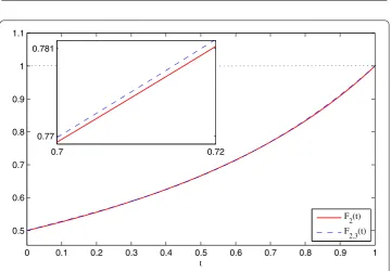
Figure 1 The comparison betweenF1(t) andF1,3(t) for Example 1.Show the accuracy of the solution functionsF1(t) andF1,3(t), respectively with exact solutions. As shown, the difference between the exact solution and the computed solution is dispensable.
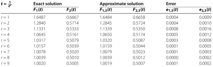
Table 1 Numerical results with error analysis for Example 1
t=21r Exact solution Approximate solution Error
F1(t) F2(t) F1,3(t) F2,3(t) e1,3(t) e2,3(t)
r= 1 1.6487 0.6667 1.6484 0.6658 0.0004 0.0009
r= 2 1.2840 0.5714 1.2845 0.5724 0.0004 0.0010
r= 3 1.1331 0.5333 1.1339 0.5350 0.0008 0.0016
r= 4 1.0645 0.5161 1.0650 0.5174 0.0005 0.0012
r= 5 1.0317 0.5079 1.0320 0.5087 0.0003 0.0008
r= 6 1.0157 0.5039 1.0159 0.5044 0.0001 0.0005
r= 7 1.0078 0.5020 1.0079 0.5023 0.0001 0.0003
r= 8 1.0039 0.5010 1.0039 0.5012 0.0000 0.0002
r= 9 1.0020 0.5005 1.0019 0.5007 0.0001 0.0002
Table 2 Absolute errors for Example 1
t= 1
2r Presented method ANN method TQR
e1,4(t) e2,4(t) e1,4(t) e2,4(t) e1,4(t) e2,4(t)
r= 1 3.50×10⁻⁶ 1.17×10⁻⁵ 7.32×10⁻⁴ 3.84×10⁻⁴ 4.11×10⁻⁴ 7.35×10⁻⁴
r= 2 2.90×10⁻⁶ 1.06×10⁻⁵ 1.15×10⁻⁴ 5.62×10⁻⁴ 3.81×10⁻⁴ 5.14×10⁻⁴
r= 3 4.78×10⁻⁵ 2.50×10⁻⁴ 5.34×10⁻⁴ 6.11×10⁻⁴ 1.29×10⁻² 8.41×10⁻⁴
r= 4 5.03×10⁻⁵ 2.50×10⁻⁴ 6.71×10⁻⁴ 6.30×10⁻⁴ 4.17×10⁻³ 3.28×10⁻³
r= 5 3.71×10⁻⁵ 1.63×10⁻⁴ 9.80×10⁻⁴ 3.27×10⁻⁴ 2.08×10⁻³ 8.20×10⁻⁴
r= 6 2.53×10⁻⁵ 8.90×10⁻⁵ 1.17×10⁻⁴ 4.83×10⁻⁴ 3.27×10⁻³ 3.53×10⁻³
r= 7 1.79×10⁻⁵ 4.30×10⁻⁵ 4.15×10⁻⁴ 4.88×10⁻⁴ 1.08×10⁻² 2.71×10⁻²
r= 8 1.37×10⁻⁵ 1.77×10⁻⁵ 3.12×10⁻⁴ 4.87×10⁻⁴ 6.31×10⁻³ 3.84×10⁻⁴
r= 9 1.16×10⁻⁵ 4.30×10⁻⁶ 1.16×10⁻⁴ 4.82×10⁻⁴ 2.10×10⁻⁴ 3.84×10⁻³
with
f(t) = et– t– sin(t) –tet+ tcos(t) –tet+ tsin(t),
f(t) = –t– et+sin(t) –tet+tcos(t) +tet+ tsin(t) – .
The exact solution of the present problem is,F(t) =sin(t) andF(t) =et. Similarly, the present method is applied to approximate solution of the integral equations system. We calculate the coefficients matricesW,VandEby using Eq. () forn= as following:
W=
W(,)W(,)
W(,)W(,)
, V=
V(,)V(,)
V(,)V(,)
, E=
E
E
,
where
W(,)=
⎡ ⎢ ⎢ ⎢ ⎢ ⎢ ⎢ ⎣
–
–, , –
, –
–
–
, – – – – – –, –, –, –,, –,,
–
⎤ ⎥ ⎥ ⎥ ⎥ ⎥ ⎥ ⎦
, E=
⎡ ⎢ ⎢ ⎢ ⎢ ⎢ ⎢ ⎣
,
, , –,, –,
⎤ ⎥ ⎥ ⎥ ⎥ ⎥ ⎥ ⎦
,
W(,)=
⎡ ⎢ ⎢ ⎢ ⎢ ⎢ ⎢ ⎣
,
, ,
,
⎤ ⎥ ⎥ ⎥ ⎥ ⎥ ⎥ ⎦
W(,)=
Now by using the above matrices, the vector solution of the generalized linear system () is obtained as follows:
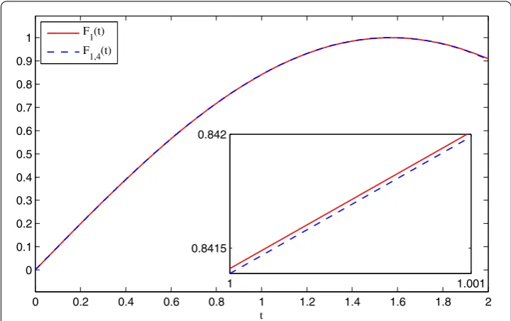
Figure 3 The comparison betweenF1(t) andF1,4(t) for Example 2.Show the accuracy of the solution functionsF1(t) andF1,4(t), respectively with exact solutions. As shown, the difference between the exact solution and the computed solution is dispensable.
Consequently, the approximate functionsF,(t) andF,(t) can be written as follows:
F,= ,t
– ,t
+ ,t
+ t,
F,= ,t
+ ,t
+ t
+, ,t+ .
Similarly, Figures and show the accuracy of the solution functionsF,(t) andF,(t), re-spectively. As shown, the difference betweenthe exact solution and the computed solution is dispensable. Similarly, numerical results can be seen in Table .
Trapezoidal rule Suppose that the region of integration is subdivided into equal in-tervals of widthh= ., integration nodesti= .ifori= , . . . , . Table illustrates the absolute values of the errors obtained here and the absolute errors of [] for this example. Furthermore, the Lagrange interpolation method has been used to design the interpola-tion polynomials.
Example Consider
⎧ ⎪ ⎪ ⎪ ⎪ ⎪ ⎪ ⎪ ⎪ ⎪ ⎪ ⎨ ⎪ ⎪ ⎪ ⎪ ⎪ ⎪ ⎪ ⎪ ⎪ ⎪ ⎩
(t+ )F
(t) =f(t) +
t
(t– s)F(s)ds+
t
(s–t)F(s)ds +tsF(s)ds,
( – t)F(t) =f(t) +
t
s(t+ )F(s)ds+
t st(t
+ )F (s)ds +t(s+t)F
(s)ds,
(t+ )F
(t) =f(t) +
t
(s–t)F(s)ds+
t
(s–t)F(s)ds +t(ts+s)F
Figure 4 The comparison betweenF2(t) andF2,4(t) for Example 2.The comparison between solution of Example 2.
Table 3 Numerical results with error analysis for Example 2
t=21r Exact solution Approximate solution Error
F1(t) F2(t) F1,4(t) F2,4(t) e1,4(t) e2,4(t)
r= 1 0.4794 1.6487 0.4795 1.6488 0.0001 0.0001
r= 2 0.2474 1.2840 0.2472 1.2825 0.0002 0.0016
r= 3 0.1247 1.1331 0.1244 1.1315 0.0003 0.0016
r= 4 0.0625 1.0645 0.0622 1.0634 0.0002 0.0011
r= 5 0.0312 1.0317 0.0311 1.0311 0.0001 0.0006
r= 6 0.0156 1.0157 0.0156 1.0154 0.0001 0.0003
r= 7 0.0078 1.0078 0.0078 1.0077 0.0001 0.0002
r= 8 0.0039 1.0039 0.0039 1.0038 0.0001 0.0001
r= 9 0.0020 1.0020 0.0019 1.0019 0.0001 0.0001
Table 4 Absolute errors for Example 2
t= 1
2r Presented method ANN method TQR
e1,5(t) e2,5(t) e1,5(t) e2,5(t) e1,5(t) e2,5(t)
r= 1 2.66×10⁻⁵ 4.92×10⁻⁵ 1.16×10⁻² 9.28×10⁻⁴ 8.32×10⁻³ 8.07×10⁻³
r= 2 5.85×10⁻⁵ 1.37×10⁻⁵ 4.30×10⁻³ 1.48×10⁻³ 2.14×10⁻² 4.81×10⁻³
r= 3 8.55×10⁻⁵ 2.04×10⁻⁵ 2.04×10⁻³ 4.43×10⁻³ 3.01×10⁻² 3.71×10⁻²
r= 4 6.14×10⁻⁵ 4.11×10⁻⁵ 1.73×10⁻³ 5.91×10⁻³ 3.91×10⁻² 3.16×10⁻²
r= 5 3.89×10⁻⁵ 9.44×10⁻⁵ 8.01×10⁻⁴ 7.94×10⁻³ 1.12×10⁻¹ 4.24×10⁻¹
r= 6 2.12×10⁻⁵ 5.17×10⁻⁵ 6.23×10⁻⁴ 1.94×10⁻² 3.62×10⁻¹ 2.80×10⁻¹
r= 7 1.11×10⁻⁵ 2.71×10⁻⁵ 5.37×10⁻⁴ 4.13×10⁻² 8.54×10⁻² 1.78×10⁻¹
r= 8 5.70×10⁻⁶ 1.38×10⁻⁵ 4.95×10⁻⁴ 6.89×10⁻² 6.37×10⁻² 7.07×10⁻²
Table 5 Numerical results with error analysis for Example 3
t=21r Exact solution Approximate solution Error
F1(t) F2(t) F3(t) F1,3(t) F2,3(t) F3,3(t) e1,3(t),i= 1,. . ., 3
r= 1 10.500 –4.5000 1.7500 10.500 –4.5000 1.7500 0.0000
r= 2 9.2500 –4.8750 1.3125 9.2500 –4.8750 1.3125 0.0000
r= 3 8.6250 –4.9688 1.1406 8.6250 –4.9688 1.1406 0.0000
r= 4 8.3125 –4.9922 1.0664 8.3125 –4.9922 1.0664 0.0000
r= 5 8.1563 –4.9980 1.0322 8.1563 –4.9980 1.0322 0.0000
r= 6 8.0781 –4.9995 1.0159 8.0781 –4.9995 1.0159 0.0000
r= 7 8.0391 –4.9999 1.0079 8.0391 –4.9999 1.0079 0.0000
r= 8 8.0195 –5.0000 1.0039 8.0195 –5.0000 1.0039 0.0000
r= 9 8.0098 –5.0000 1.0020 8.0098 –5.0000 1.0020 0.0000
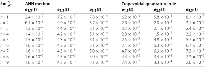
Table 6 Absolute errors for Example 3
t=21r ANN method Trapezoidal quadrature rule
e1,3(t) e2,3(t) e3,3(t) e1,3(t) e2,3(t) e3,3(t)
r= 1 2.4×10⁻² 7.2×10⁻³ 7.8×10⁻⁴ 6.2×10⁻³ 5.8×10⁻³ 8.1×10⁻³
r= 2 6.1×10⁻³ 4.9×10⁻³ 5.7×10⁻⁴ 2.0×10⁻² 2.0×10⁻² 2.1×10⁻²
r= 3 1.3×10⁻² 4.4×10⁻³ 5.1×10⁻⁴ 3.7×10⁻² 2.1×10⁻² 2.4×10⁻²
r= 4 1.4×10⁻² 4.2×10⁻³ 5.1×10⁻⁴ 2.8×10⁻² 1.5×10⁻² 3.2×10⁻²
r= 5 1.5×10⁻² 4.3×10⁻³ 5.1×10⁻⁴ 2.5×10⁻³ 4.8×10⁻³ 5.7×10⁻³
r= 6 1.6×10⁻² 4.2×10⁻³ 5.1×10⁻⁴ 2.1×10⁻² 5.3×10⁻² 6.7×10⁻³
r= 7 1.6×10⁻² 4.3×10⁻³ 5.0×10⁻⁴ 4.7×10⁻² 6.9×10⁻³ 7.3×10⁻³
r= 8 1.6×10⁻² 4.3×10⁻³ 5.0×10⁻⁴ 4.3×10⁻² 3.4×10⁻² 2.2×10⁻²
r= 9 1.6×10⁻² 4.3×10⁻³ 5.1×10⁻⁴ 2.4×10⁻² 3.3×10⁻⁴ 2.6×10⁻²
where
f(t) = –
t+ t– t– t– t– , f(t) = –
t+ t– t+ t+ t– t+ , f(t) =
t– t– t+ t+ t+ t+ ,
with the exact solution,F(t) = t+ ,F(t) = t– andF(t) =t+t+ . Again,we solved this example by this method and the results are given in Table . Table illustrates the absolute errors of ANN method and TQR for this example.
As we can see this method will be useful when the exact solution is a polynomial. In other word, the proposed method give the analytical solution for the system, if the exact solution be polynomials of degreenor less thann.
5 Conclusions
Additionally, the proposed method has been compared with ANN method [] and TQR. The analyzed examples illustrated the ability and reliability of the present method. The obtained solutions, in comparison with exact solutions admit a remarkable accuracy. Ex-tensions to the case of more general systems of integral equations are left for future studies.
Competing interests
The authors declare that they have no competing interests.
Authors’ contributions
The authors have equal contributions and they have approved the final version of the manuscript.
Author details
1Department of Mathematics, Urmia Branch, Islamic Azad University, Urmia, Iran.2Department of Physics, Urmia Branch,
Islamic Azad University, Urmia, Iran. 3Department of Mathematics and Computer Sciences, Faculty of Art and Sciences,
Çankaya University, Balgat, Ankara, 0630, Turkey.4Department of Chemical and Materials Engineering, Faculty of
Engineering, King Abdulaziz University, P.O. Box 80204, Jeddah, 21589, Saudi Arabia.5Institute of Space Sciences, P.O. Box
MG-23, Magurele, Bucharest 76900, Romania.
Acknowledgements
We would like to thank the referees for their comments and remarks.
Received: 30 January 2013 Accepted: 8 April 2013 Published: 2 May 2013
References
1. Tricomi, FG: Integral Equations. Dover, New York (1982)
2. Lan, X: Variational iteration method for solving integral equations. Comput. Math. Appl.54, 1071-1078 (2007) 3. Babolian, E, Sadeghi Goghary, S, Abbasbandy, S: Numerical solution of linear Fredholm fuzzy integral equations of
the second kind by Adomian method. Appl. Math. Comput.161, 733-744 (2005)
4. Liao, SJ: Beyond Perturbation: Introduction to the Homotopy Analysis Method. Chapman & Hall/CRC Press, Boca Raton (2003)
5. Abbasbandy, S: Numerical solution of integral equation: homotopy perturbation method and Adomian’s decomposition method. Appl. Math. Comput.173, 493-500 (2006)
6. Kanwal, RP, Liu, KC: A Taylor expansion approach for solving integral equations. Int. J. Math. Educ. Sci. Technol.2, 411-414 (1989)
7. Maleknejad, K, Aghazadeh, N: Numerical solution of Volterra integral equations of the second kind with convolution kernel by using Taylor-series expansion method. Appl. Math. Comput.161, 915-922 (2005)
8. Nas, S, Yalcynbas, S, Sezer, M: A Taylor polynomial approach for solving high-order linear Fredholm integrodifferential equations. Int. J. Math. Educ. Sci. Technol.31, 213-225 (2000)
9. Babolian, E, Masouri, Z, Hatamzadeh-Varmazyar, S: A direct method for numerically solving integral equations system using orthogonal triangular functions. Int. J. Ind. Math.2, 135-145 (2009)
10. Jafari, H, Hosseinzadeh, H, Mohamadzadeh, S: Numerical solution of system of linear integral equations by using Legendre wavelets. Int. J. Open Probl. Comput. Sci. Math.5, 63-71 (2010)
11. Bhatti, MI, Bracken, P: Solutions of differential equations in a Bernstein polynomial basis. J. Comput. Appl. Math. (2007). doi:10.1016/j.cam.2006.05.002
12. Farouki, RT, Goodman, TNT: On the optimal stability of the Bernstein basis. Math. Comput.65(216), 1553-1566 (1996) 13. Yousefi, SA, Behroozifar, M: Operational matrices of Bernstein polynomials and their applications. Int. J. Syst. Sci.41(6),
709-716 (2010)
14. Bhatta, DD, Bhatti, MI: Numerical solution of KdV equation using modified Bernstein polynomials. Appl. Math. Comput.174, 1255-1268 (2006)
15. Mandal, BN, Bhattachary, S: Numerical solution of some classes of integral equations using Bernstein polynomials. Appl. Math. Comput.191, 1707-1716 (2007)
16. Bhattacharya, S, Mandal, BN: Use of Bernstein polynomials in numerical solution of Volterra integral equations. Appl. Math. Sci.6, 1773-1787 (2008)
17. Maleknejad, K, Hashemizadeh, E, Ezzati, R: A new approach to the numerical solution of Volterra integral equations by using Bernstein’s approximation. Commun. Nonlinear Sci. Numer. Simul.161, 647-655 (2011)
18. Jafarian, A, Measoomy, NS: Utilizing feed-back neural network approach for solving linear Fredholm integral equations system. Appl. Math. Model. (2012). doi:10.1016/j.apm.2012.09.029
19. Hochstadt, H: Integral Equations. Wiley, New York (1973)
doi:10.1186/1687-1847-2013-123