R E S E A R C H
Open Access
Legendre-Gauss collocation methods for
nonlinear neutral delay differential equations
Jingjun Zhao, Yang Cao and Yang Xu
**Correspondence:
Department of Mathematics, Harbin Institute of Technology, Harbin, 150001, China
Abstract
In this paper, an efficient Legendre-Gauss collocation method is introduced for solving nonlinear neutral delay differential equations (NDDEs). Firstly, the single-step Legendre-Gauss collocation method is presented for NDDEs; we analyze the convergence of the method with different delay functions. Then the multi-domain Legendre-Gauss collocation method is presented, which is based on the single-step one; the results of convergence are also obtained. In addition, numerical results are presented to confirm our analysis.
Keywords: Legendre-Gauss collocation methods; nonlinear neutral delay differential equations; spectral accuracy
1 Introduction
Delay differential equations (DDEs) arise in a variety of fields such as biology, economics, control theory, and so on (see [–]). In particular, neutral delay differential equations (NDDEs) provide an important mathematical instrument to model several electromag-netic problems [].
Recently, much literature has been devoted to the numerical solutions of NDDEs (see [–]). Meanwhile, a Legendre-tau method was proposed and analyzed for linear DDEs with one constant delay in []. The Legendre-Gauss collocation methods were studied for ordinary differential equations (ODEs) based on the Legendre polynomial expansions in [, ]. Moreover, the Legendre-Gauss collocation methods were developed for nonlinear DDEs in []. Wang and Guo proposed an efficient numerical integration process for initial value problems of first order ODEs, based on the Legendre-Gauss-Radau interpolation, which is easy to implement and possesses the spectral accuracy in []. However, it is more interesting but challenging to develop and analyze the type of high-order methods for nonlinear NDDEs of the form
U(t) =f(t,U(t),W(t),dtdW(t)), ≤t≤T,
U(t) =V(t), t≤, ()
whereW(t) =U(θ(t)),f,θ, andVare given functions.
If the initial functionV(t) does not link smoothly with the solutionU(t) at , this discon-tinuity point is spread forward on a set of primary discondiscon-tinuity points where the solution, unlike the non-neutral case, remains solely of classC[].
The question is crucial of how to deal with the primary discontinuity points. Firstly, we assume thatT is very small such that there is no primary discontinuity point on [,T], then a single-step scheme for () is constructed. The scheme has an infinite order of accu-racy both in time and delay variable. On the basis of the single-step scheme, we partition [,T] into several subintervals, and construct multi-domain scheme on [,T], on which there are primary discontinuity points. The multi-domain scheme enjoys remarkable ad-vantages over the Runge-Kutta type methods, since the approximate solution ofU(t) is
C∞-continuous in the interior of each subinterval iff,θ,VareC∞-continuous []. The paper is organized as follows. In Section , we present and analyze the single-step Legendre-Gauss collocation method with three different delay termsθ(t) on [,T], where
T is small enough, and we provide some numerical results to justify our theoretical anal-ysis. In Section , the multi-domain version is described on [,T], on which there exist primary discontinuity points, and the convergence results are also derived. Some numer-ical results justify our theoretnumer-ical analysis.
2 The single-step Legendre-Gauss collocation method
In this section, we describe and analyze a single-step numerical process for the NDDE () using the Legendre-Gauss interpolation when there is no discontinuous point on [,T]. The single-step scheme serves as a base for the multi-domain one to be presented in the forthcoming section, which is suitable for the situation with discontinuous points.
2.1 Preliminaries
LetLl(t) be the standard Legendre polynomial of degreel. The shifted Legendre polyno-mials are defined by (see [])
LT,l(t) =Ll
t T –
=(–)
l
l! ∂ l t
tl
– t
T
l
, l= , , , . . . .
According to the properties of the standard Legendre polynomials, we have
(l+ )LT,l+(t) – (l+ )
t T –
LT,l(t) +lLT,l–(t) = , l≥, ()
d
dtLT,l+(t) – d
dtLT,l–(t) =
T(l+ )LT,l(t), l≥, ()
LT,l(t)≤, t∈[,T],l≥. ()
The set ofLT,l(t) is a completeL(,T)-orthogonal system, namely,
T
LT,l(t)LT,m(t)dt=
T
l+δl,m, whereδl,mis the Kronecker symbol. Thus, for anyv∈L
(,T),v(t) =∞
l=vˆT,lLT,l andvˆT,l=lT+
T
v(t)LT,l(t)dt.
Now, we introduce the shifted Legendre-Gauss interpolation. Denote the nodes of the standard Legendre-Gauss interpolation on the interval [–, ) bytN
j (≤j≤N). In par-ticular,tN = –. The corresponding Christoffel numbers areωNj (≤j≤N). The nodes of the shifted Legendre-Gauss interpolation on the interval [,T) are the distinct zeros of
LetPN(,T) be the set of polynomials of degree at mostN. Due to the property of the standard Legendre-Gauss quadrature, it follows that, for anyφ∈PN(,T), one has
T
φ(t)dt=T
N
j= ωNj φ
T
tjN+ = N
j=
ωTN,jφtNT,j. ()
Let (u,v)TandvTbe the inner product and the norm of spaceL(,T), respectively. We also introduce the following discrete inner product and norm:
(u,v)T,N= N
j=
utTN,jvtNT,jωNT,j,
vT,N= (v,v) T,N.
According to (), for anyϕ∈PN(,T) andφ·ψ∈PN(,T), one can obtain
(φ,ψ)T= (φ,ψ)T,N, ϕT=ϕT,N. ()
For anyv∈C[,T), the shifted Legendre-Gauss interpolationIT,Nv(t)∈PN(,T) is de-termined uniquely by
IT,Nv
tNT,j=vtTN,j, ≤j≤N.
Letrbe a nonnegative integer,Hr(,T) be the usual Sobolev space as defined in [], and denote the semi-norm by| · |r,T, where|U|r,T= (
T
(d rU
dtr )dt)
andU∈Hr(,T). We
have the following estimates.
Lemma (see []) For any u∈Hr(,T)with integer≤r≤N+ ,we have
IT,Nu–uT≤cTrN–r|u|r,T, () (IT,Nu–u)T≤cTr–N
–r|u|r,T. ()
Lemma Let u∈PN+,then
uT,N≤uT. ()
Proof Letu∈PN+,u(t) =
N+
k=u˜T,kLT,k, we haveuT=
N+
k=u˜T,kkT+. Moreover,
ac-cording to () and (), we can obtain
uT,N = N+
k= ˜ uT,kLT,k,
N+
k= ˜ uT,kLT,k
T,N
= N
k= ˜
uT(LT,k,LT,k)T+ u˜T,Nu˜T,N+(LT,N,LT,N+)T,N
Due to (), we deduce that
This completes the proof.
2.2 The single-step scheme
Now, we present the single-step scheme for the NDDEs (). Denote the grid set by N=
{tN
Lagrange interpolation is not stable for largeN. Hence, we propose a more stable approach by expandinguN(t) directly in terms of the shifted Legendre polynomials and solving the unknown coefficients of the collocation scheme (). This approach is stable for largeN, and much easier to implement.
To describe the numerical implementation of the collocation scheme (), we expand the collocation solution as
uN(t) = N+
l= ˆ
uNT,lLT,l(t)∈PN+(,T), <t≤T. ()
Let [l] be the integer part ofl. According to [], we have d
dtLT,l(t) =
T [l– ]
m=(l– m–
)LT,l–m–(t) andLT,l() = (–)l. Hence, () is equivalent to
N+
l= aNT,k,luˆNT,l=fTN,k, ≤k≤N,
N+
l=(–)luˆNT,l=V(),
()
whereaN T,k,l=
T [l– ]
m=(l– m– )LT,l–m–(tNT,k), ≤k≤N, ≤l≤N+ , and
fTN,k= ⎧ ⎪ ⎪ ⎨ ⎪ ⎪ ⎩
f(tTN,k,Nl=+uˆNT,lLT,l(tNT,k), N+
l= uˆNT,lLT,l(θ(tTN,k)), d
dt N+
l= uˆNT,lLT,l(θ(t))|t=tNT,k), tTN,k∈ N,
f(tN T,k,
N+
l= uˆNT,lLT,l(tNT,k),V(θ(tTN,k)),V(θ(tNT,k))), tTN,k∈ N.
LetANT be the matrix with the entriesaNT,k,l, ≤k≤N, ≤l≤N+ . We can give the matrix form for () as follows:
AN
TuˆNT =FTN(uˆNT),
ˆ uN
T,=V() –
N+
l= (–)luˆNT,l,
()
whereuˆNT= (uˆNT,,uˆNT,, . . . ,uˆNT,N+),FTN(uˆNT) = (fTN,,fTN,, . . . ,fTN,N). In fact, () is a set of lin-ear equations about {ˆuNT,l}Nl=+. Therefore, we can solve () and recover the collocation solutionuN(t), <t≤Tfrom ().
2.3 Error analysis
In this subsection, we shall analyze the convergence of the scheme () with three assump-tions of delay functionθ(t), respectively. In particular, we prove the spectral accuracy of the numerical solutionuN(t). LetI
T,N be the Legendre-Gauss interpolation operator as defined before. LetEN(t) =uN(t) –I
T,NU(t) andGNT,(t) =IT,NdtdU(t) –dtdIT,NU(t). Ac-cording to (), we have
d
dtIT,NU(t) =f
t,U(t),W(t),W(t)–GNT,(t), t∈ N. ()
Subtracting () from (), we obtain
d
dtEN(t) =GNT,(t) +GNT,(t), t∈ N,
EN() =U() –I
T,NU(),
()
whereGNT,(t) =f(t,uN(t),w(t),w(t)) –f(t,I
Lemma Let U and uN be the solutions of()and(),respectively,U∈Hr(,T)with
integer≤r≤N+ ,then
t
–EN–EN()
T+T
–EN(T) –EN()≤
d
dtE
N(t)
T,N
. ()
Proof Due to the proof of Lemma in [], we have
EN–EN(), d
dt
t–EN–EN() T,N
= –t–EN–EN()T+T–EN(T) –EN().
On the other hand, we derive that
d dt
t–EN(t) –EN()= –t–EN(t) –EN()+t–d dtE
N(t), t∈ N.
Hence, by (), we deduce that
EN–EN(), d
dt
t–EN–EN() T,N
≤–t–EN–EN() T+
t
–EN–EN() T+
dtdEN
T,N .
This completes the proof.
Now, we consider three cases according to the delay terms and analyze the numerical errors. Here,β,β, andβdenote any positive numbers less than.
Case . Consider () with the following delay:
θ(t) =λt, <λ≤. ()
In this situation, no values ofU(t) are needed in the delay term behind , therefore, no discontinuities propagate from . Then the solution is regular according to the regularity off andθ.
Assume thatf(t,x,y,z) satisfies the following Lipschitz conditions inx,y, andz. That is, there exist real numbersr≥,r≥, and ≤r<√λsuch that
f(t,x,y,z) –f(t,x,y,z)≤r|x–x|, ()
f(t,x,y,z) –f(t,x,y,z)≤r|y–y|, ()
f(t,x,y,z) –f(t,x,y,z)≤r|z–z|. ()
Theorem Consider the NDDE(),where f(t,x,y,z)is Cr-continuous in[,T]×Rd×
U∈Hr(,T)with≤r≤N+ ,and,for certainδ,δ
depending only onβ.
Proof Obviously, in this case,
N=∅. Denote
Applying (), we have
+ ( +δ)( +δ˜) +δˆ–rλd
dt(IT,NU–U)
T
+cTr–N–r|U|r,T
≤( +δ)( +δ˜)( +δˆ)rλd dtE
N
T
+cTr–N–r|U|r,T.
By (), we have
dtdEN
T,N
≤( +δ)GNT,
T,N+
+δ– GNT,T,N
≤( +δ)( +δ˜)( +δˆ)( +δ)λr
dtdEN
T,N +cTr–N–r|U|r,T+ ( +δ)G˜NT,
T,N + +δ– GNT,T,N,
where
GNT,T,N =GNT,T
≤( +δ)d
dt(IT,NU–U)
T
+ +δ–IT,N
d dtU–
d dtU
T
≤cTr–N–r|U|r,T.
The above fact leads to
dtdEN
T,N
≤( +δ) ˆ c G˜
N T,
T,N+cT
r–N–r|U|
r,T,
wherecˆ= – ( +δ)( +δ˜)( +δˆ)( +δ)λr.
Let us estimate ˜GNT,T,N. Clearly, by () and ()-(), we have
G˜NT,T,N ≤ +δ–( +δ)rEN
T,N
+ +δ– +δ–rw(t) –IT,NW(t)T,N
≤ +δ–( +δ)rEN
T
+ +δ– +δ–rw(t) –IT,NW(t)
T,
where
w(t) –IT,NW(t)T
≤( +ε)w(t) –W(t)T+ +ε–W(t) –IT,NW(t)T
≤( +ε)
T
uNθ(t)–Uθ(t)dt+cε–TrN–r|U|r,T
Thus, we can obtain
G˜NT,T,N ≤ +δ–( +δ)rEN
T
+ +δ– +δ–( +ε)λ–ruN–UT
+cε–Tr–N–r|U|r,T.
According to (), we have
t
–EN–EN()
T+T
–EN(T) –EN()
≤( +δ)( +δ–)( +δ)r ˆ
c E
N
T
+( +δ)( +δ
–)( +δ–
)( +ε)λ–r ˆ
c u
N–U T
+cε–TrN–r|U|r,T.
Moreover, we can obtain
ENT≤( +ε)Tt–EN–EN()T+ +ε–EN()T
and
E
N
T+ ( +ε)TE
N(T) –EN()
≤( +ε)T
t
–EN–EN() T+T
–EN(T) –EN()
+cε–TEN()
≤( +ε)( +δ)( +δ–)( +δ)Tr ˆ
c E
N
T
+( +δ)( +δ
–)( +δ–
)( +ε)Tλ–r ˆ
c u
N–U T
+cε–TrN–r|U|r,T+cε–TEN().
Thanks to (), we have
U–uNT≤( +ε)ENT + +ε–U–IT,NUT
≤( +ε)ENT+cε–TrN–r|U|r,T.
The above result yields
–
( +ε)( +δ)( +δ–)( +δ)Tr ˆ
c
U–uNT
+ ( +ε)TEN(T) –EN()
≤( +ε)( +δ)( +δ–)( +δ–)λ–Tr ˆ
c u
N–U
T
+cε–TrN–r|U|r,T+cε–TEN().
Letε= (β)/– > , then ( +ε)β=
. Thus, we can obtain
ˆ
q = ( +δ)( +δ
–)T(( +ε)( +δ
)r+ ( +ε)( +δ–)λ–r)
– ( +δ)( +δ)( +δ˜)( +δˆ)λr
< ( +ε)( +δ)( +δ
–)T(( +δ
)r+ ( +δ–)λ–r)
– ( +δ)( +δ)( +δ˜)( +δˆ)λr
≤( +ε)β= .
By a combination of the above estimates, we deduce that U–uNT≤cβTrN–r|U|r,T,
EN(T)≤EN(T) –EN()+ EN()≤cβTr–N–r|U|r,T,
wherecβ= cε – –ˆq
. Consequently, we have
U(T) –uN(T)≤IT,NU(T) –U(T)
+ EN(T)
≤cβTr–N–r|U|r,T,
dtdU–uN
T
≤d
dtE
N
T + d
dt(U–IT,NU)
T
≤cβTr–N–r|U|r,T.
From (.) of [], it can be seen thatmaxt∈[,T]|v(t)|≤ TvT+ Tdvdt
T for anyv∈
H(,T). Hence, we deduce thatmax
t∈[,T]|U(t) –uN(t)|≤cβTr–N–r|U|r,T.
Remark For () and () without the neutral term, the convergence results are the same as Case I in [].
Remark The condition () is necessary for the proof, but it is not sufficient. Some nu-merical examples do not satisfy this condition, but the nunu-merical scheme still converges. This remark also applies to the multiple-domain case.
Case . Assume that the delay functionθ(t) satisfies
θ(t) =t–τ, τ> ,t∈[,T]. ()
In this situation, the pointstk=kτ (k= , , . . .) are primary discontinuity points. There-fore, there is no discontinuity point when T ≤ τ. Moreover, f(t,x,y,z) satisfies the Lipschitz conditions ()-(), wherersatisfies ≤r< .
Theorem Consider the NDDE() with T ≤τ, where f(t,x,y,z) is Cr-continuous in [,T]×Rd×Rd×Rd,and the initial function V(t)is Cr-continuous. If the conditions
()-()and()hold,U∈Hr(,T)with integer≤r≤N+ , ( +δ)Tr
≤β< , and(T–τ)(+δ)(+δ–)((+δ)r+(+δ– )r)
–(+δ)(+δ)(+δˆ)(+δ˜)r ≤
β< for certainδ,δ,δ,δˆ,δ˜> ,then we have
U–uNT≤cβ,βT
rN–r|U|
r,T, U(T) –uN(T)≤cβ,βT
r–N–r|U|
r,T.
In particular,maxt∈[,T]|U(t) –uN(t)|≤cβ,βTr–N–r|U|r,T,where cβ,β is a positive
constant depending only onβ,β.
Proof Asτ ≥T,θ(t) < fort∈[,T]. In this case,
N =∅. Hence, by virtue of (), we haveGNT,T,N≤rENT,N. Due to () and (), we derive that
– ( +ε)( +δ)T
r
ENT+ ( +ε)TEN(T) –EN()
≤cε–TrN–r|U|r,T.
Letε= (
β) > , then
ˆ
q= ( +ε)( +δ)Tr< ( +ε)β= /.
Thus,
ENT≤cβT
rN–r|U|
r,T
and
U–uNT≤( +ε)ENT + +ε–U–IT,NUT
≤cβT
rN–r|U|
r,T, U(T) –uN(T)≤IT,NU(T) –U(T)
+ EN(T)
≤cβT
r–N–r|U|
r,T,
dtdU–uN
T
≤d
dtE
N
T + d
dt(U–IT,NU)
T
≤cβT
r–N–r|U|
r,T,
max
t∈[,T]
U(t) –uN(t)≤cβT
r–N–r|U|
r,T,
wherecβ= cε–
–qˆ.
Case . Assume that the delay functionθ(t) satisfies ⎧
⎪ ⎨ ⎪ ⎩
D:θ(t) =t–τ(t), τ∈Cd(I),d≥;
D:τ(t)≥τ> , t∈I; D:θis strictly increasing onI.
()
Now, we assume that{Tk}∞k=are primary discontinuity points which satisfyθ(tk+) =tk, t= . By the definition ofθ(t), we conclude thattk+≥tk+τ,k= , , . . . . WhenT≤t,
there is no discontinuity point.
Moreover, the functionf(t,x,y,z) satisfies the Lipschitz conditions ()-(), butr sat-isfies ≤r<√
c, wherec=maxt∈[,T]
Theorem Consider the NDDE () with T ≤t which satisfy θ(t) = .f(t,x,y,z) is Cr-continuous in[,T]×Rd×Rd×Rd,and the initial function V(t)is Cr-continuous.
If the conditions ()-()and()hold,U ∈Hr(,T)with integer≤r≤N+ , c
= mint∈[,T][θ–(t)], ( +δ)Tr ≤β<and
( +δ)( +δ–)( +δ)Tr+ ( +δ)( +δ–)( +δ– )cTr
– ( +δ)( +δ)( +δˆ)( +δ˜)cr
≤β<
for certain δ,δ,δ,δˆ,δ˜> ,then we have().In particular,maxt∈[,T]|U(t) –uN(t)|≤ cβ,βTr–N–r|U|r,T,where cβ,β is a positive constant depending only onβ,β.
Proof Together with () andθ() < , we can findtwhich satisfiesθ(t) = . Let
N={tNT,k|θ(tTN,k) < , ≤k≤N},
N={tNT,k|≤θ(tNT,k)≤T, ≤k≤N}.
Ift≥T, obviously, N=∅. The proof is similar toτ≥Tin Case ., thus we have U–uNT≤cβT
rN–r|U|
r,T, U(T) –uN(T)
≤cβT
r–N–r|U|
r,T,
max
t∈[,T]
U(t) –uN(t)≤cβT
r–N–r|U|
r,T.
2.4 Numerical results
In this subsection, we give some numerical results to illustrate the efficiency of our single-step algorithm.
Example Consider the following equation:
d dtu(t) =
u(t) +
e
t
u(t
) + e
t
u(t
), ≤t≤T,
u() = . ()
The exact solution isu(t) =et. Obviously, the conditions ()-() hold withr= ,r=
e T
, andr=
e T
.
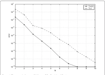
Moreover, the inequality () is satisfied forT= .. But it is no longer valid forT= . In Figure , we plot the numerical errors att=T forT = . andT= , respectively. It indicates that the numerical errors decay exponentially asNincreases. In particular, we can observe that our algorithm is still valid even if the condition () is not satisfied.
Example Consider the following equation:
⎧ ⎪ ⎨ ⎪ ⎩ d dtu(t) =
u(t) +
e
u(t–
) + e
u(t–
), ≤t≤T, u(t) =et, t< ,
u() = .
()
The exact solution isu(t) =et. Obviously, the conditions ()-() hold withr=,r=
e
, andr=
e
Figure 1 The numerical errors of (25) att=TforT= 0.3 andT= 1.
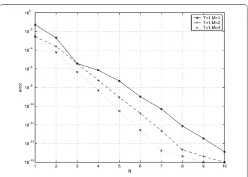
Figure 2 The numerical errors of (26) or (27) att=TforT= 0.125 andT= 0.5.
Moreover, the inequality Tr
≤β<in Theorem is satisfied forT= .. But it is
no longer valid forT= .. In Figure , we plot the numerical errors att=TforT= . andT= ., respectively. It indicates that the numerical errors decay exponentially asN
Example Consider the following equation:
⎧ ⎪ ⎨ ⎪ ⎩ d dtu(t) =
u(t) +
e
t+
u(θ(t)) +
e t+
u(θ(t)), ≤t≤T,
u(t) =et, t< ,
u() = ,
()
whereθ(t) =t– (t
+
). The exact solution isu(t) =e
t. Obviously, the conditions ()-()
hold withr=,r=eT+, andr=
e T+
. The discrete scheme of () is the same as ().
So, we can also see the convergence of numerical solution of this equation in Figure . Here, the inequality Tr
≤β< in Theorem is satisfied forT = .. But it is no
longer valid forT= .. In Figure , we plot the numerical errors att=T forT= . andT= ., respectively. It indicates that the numerical errors decay exponentially asN
increases. In particular, we can observe that our algorithm is still valid even if the above inequality is not satisfied.
3 The multiple-domain Legendre-Gauss collocation method
We investigate the single-step Legendre-Gauss collocation method in Section . The nu-merical errors decay very rapidly asNandrincrease. While the single-step collocation method provides accurate results, it is not suitable for resolving the discrete system () with largeT. When there are some discontinuity points on [,T], the single-step method cannot be employed. We shall partition the interval [,T] into a finite number of subin-tervals by a set of points{Tk}Mk=. The primary discontinuity points on [,T] should be all contained in the set of{Tk}Mk=such that the solutionU(t) is continuous in the interior of
each subinterval. Then we solve the equations subsequently on each subinterval.
3.1 The multiple-domain scheme
Now, we describe the multiple-domain scheme. LetMandNm, ≤m≤Mbe any positive integers. Decompose the interval [,T] intoMsubintervals [Tm–,Tm], ≤m≤M, such that the set ofTmincludes all breaking points, whereT= andTM=T. Letτm=Tm–
Tm–, ≤m≤M. We shall useuNmm(t)∈PNm+(,τm) to approximate the solutionUin the
subinterval [Tm–,Tm].
Firstly, replacingTandNbyτandNin () and all other formulas in Section ., we
can derive an alternative algorithm, with which we obtain the numerical solutionuN
∈ PN+(,τ). Then we evaluate the numerical solutionsuNmm ∈PNm+(,τm), ≤m≤M,
step by step. Finally, the global numerical solution of () is given by
uN(Tm–+t) =uNmm(t), ≤t≤τm, ≤m≤M. ()
We present the numerical scheme foruNm
m (t). Denote the nodes and the corresponding Christoffel numbers of the shifted Legendre-Gauss interpolation on the interval (,τm) by
tNm
τm,kandω Nm
τm,k, ≤k≤Nm, respectively. Let
N,m={t Nm
τm,k|θ(Tm–+t
Nm
τm,k) < , ≤k≤Nm},
j N,m={t
Nm
τm,k|θ(Tm–+t Nm
The multiple-domain collocation method for () is to seekuNm
It can be seen from () and () that the local numerical solutionuNm
m (t) is actually an approximation to the local exact solutionUm(t), with the approximate initial datauNm
m () =
uNm– m– (τm–). 3.2 Error analysis
We now analyze the numerical errors. LetENm
Lemma Let uNm
Proof Applying Lemma , we have
d
This completes the proof.
We shall analyze the numerical errors in the following three cases. Letτˆ=max≤j≤Mτj andN=min≤j≤MNj. Assume that, for any ≤i≤j≤M,τi/τjis bounded.
Case . Consider the delay function θ(t) satisfying the condition (). The solution
then,for any≤m≤M,we have
stant depending only onβ.
Proof Clearly, in this case,
By (), we have
It can be found that
Applying Lemma , we deduce that
discon-Then we can obtain satisfies the Lipschitz conditions ()-(), but r satisfies ≤r < √
(III) IfTm–<t≤Tm, then we decompose the interval [,τm] into [,t–Tm–] and
[t–Tm–,τm]. Denoteτm,=t–Tm–andτm,=τm– (t–Tm–), we shall useuNmm,∈ PNm+(,τm,) anduNmm,∈PNm+(,τm,) to approximate the solutionUin the subinterval
[,τm,] and [τm,,τm], respectively.
The global numerical solution of () is given by
uN(Tm–+t) =uNmm(t) =u Nm
m,(t), ≤t≤τm,,
uN(Tm–+τm,+t) =uNmm(τm,+t) =uNmm,(t), ≤t≤τm,.
LetUm,(t) =Um(t) =U(Tm–+t) fort∈[,τm,] andUm,(t) =Um(τm,+t) =U(Tm–+ τm,+t) fort∈[,τm,].
Firstly, we seekuNm
m,∈PN+(,τm,). Obviously, jN,m=∅(≤j≤m). The proof is similar to the case oft>Tm, and we can obtain the results that
uNm
m,–Um,τ m≤cβτˆ
rN–r|U|
r,Tm,
Um,(τm,) –uNm,(τm,)
≤cβτˆ
r–N–r|U|
r,Tm,
max
t∈[,τm,]
Um,(t) –uNm,(t) ≤
cβτˆ
r–N–r|U|
r,Tm.
Then we evaluateuNm
m,∈PNm+(,τm,). Obviously, N,m=∅, the proof is similar tot<
Tm–. Therefore, we can obtain
uNm
m,–Um,τ
m,≤cβτˆ
rN–r|U|
r,Tm,
Um,(τm,) –uNm,(τm,)
≤cβτˆ
r–N–r|U|
r,Tm,
max
t∈[,τm,]
Um,(t) –uNm,(t)
≤cβτˆ
r–N–r|U|
r,Tm.
Thus, we can obtain the results of Theorem .
3.3 Numerical results
In this subsection, we give some numerical results to illustrate the efficiency of our multiple-domain algorithm.
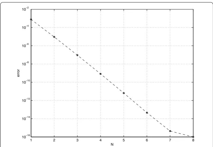
Example Consider () by multiple-domain algorithm. Firstly, we decompose the inter-val [,T] withT= . into two intervals with uniformτm= . andNm=N,m= , . We plot the numerical errors att= . in Figure , which indicates that the numerical errors decay exponentially asN increases. Then we consider () withT = and decompose equally the interval [,T] intoM= , and subintervals, respectively. The inequality () is satisfied forM= , but forM= andM= , the inequality () is no longer valid. Figure indicates that the numerical errors decay exponentially asNm=Nincreases and
τmdecreases,m= , . . . ,M. In particular, it can be observed from Figure that even if the condition () is not satisfied, our multiple-domain algorithm is still valid (see the cases ofM= , ).
Figure 3 The numerical errors of (25) att=T= 0.5 with uniformτm= 0.25,m= 1, 2.
Figure 5 The numerical errors of (26) or (27) att=T= 0.5 with uniformτm= 0.25,m= 1, 2.
Example Consider () by multiple-domain algorithm. To consider (), we use multiple-domain method at t=T = . with uniformτm = . andNm=N,m= , . The multiple-domain discrete scheme of () is the same as (). So, we can also see the convergence of the numerical solution of this equation in Figure .
Example Consider the following equation: ⎧
⎪ ⎨ ⎪ ⎩ d
dtu(t) = –u
(t– ), ≤t≤,
u(t) =t, –≤t≤,
u() = .
()
The exact solution is
u(t) = ⎧ ⎪ ⎨ ⎪ ⎩
–t, ≤t≤,
t– , ≤t≤, –t, ≤t≤,
()
where , , , are primary discontinuity points. To consider the equation (), we use multiple-domain method atT= with uniformτm≡ andNm=N(m= , , ). For the linear property of (), the approximate solution is equal to () on each subinterval. Therefore, we find that the values of the numerical error function are all zero at point
t= , , withNm= , . . . , (m= , , ). So, the multiple-domain method is efficient and accurate.
4 Conclusions
(I) We can use moderateNto evaluate the numerical solutions more effectively by using the multiple-domain Legendre-Gauss collocation method. We benefit from the orthogo-nality of Legendre polynomials, while in the derivation of algorithm of the implicit Runge-Kutta method, one used the Lagrange interpolation on the Legendre-Gauss interpolation nodes, which is not stable for largeN. In particular, our methods are much easier to be implemented than the implicit Runge-Kutta method for NDDEs, since we only need to save the coefficients of numerical solutions in each step.
(II) The numerical errors of our methods are characterized by the semi-norms of exact solutions in certain Sobolev spaces. These sharp norms are in particular necessary for the problems with degenerate initial data.
The numerical results demonstrate the spectral accuracy of proposed algorithms and coincide with the theoretical analysis very well.
Competing interests
The authors declare that they have no competing interests.
Authors’ contributions
All authors contributed equally to the writing of this paper. All authors read and approved the final manuscript.
Acknowledgements
The authors would like to thank the anonymous referees for their valuable comments, which helped us to improve the present paper. This work was supported by the National Natural Science Foundation of China (11101109, 11271102), the Natural Science Foundation of Hei-long-jiang Province of China (A201107), PIRS of HIT (A201405) and SRF for ROCS, SEM.
Received: 12 September 2014 Accepted: 25 December 2014
References
1. Weldom, TE, Kirk, J, Finlay, HM: Cyclical granulopoiesis in chronic granulocytic leukemia: a simulation study. Blood43, 379-387 (1974)
2. Brayton, RK: Small signal stability criterion for networks containing lossless transmission lines. IBM J. Res. Dev.121, 431-440 (1968)
3. Kuang, Y: Delay Differential Equations with Application in Population Dynamics. Academic Press, Boston (1993) 4. Ruehli, AE, Miekkala, U, Bellen, A, Heeb, H: Stable time domain solutions for EMC problems using PEEC circuit models.
In: Proceedings of IEEE Int. Symposium on Electromagnetic Compatibility (1994)
5. Guglielmi, N: Inexact Newton methods for the steady-state analysis of nonlinear circuits. Math. Models Methods Appl. Sci.6, 43-57 (1996)
6. Hale, JK, Verduyn Lunel, SM: Introduction to Functional Differential Equations. Springer, New York (1993)
7. Liu, Y: Numerical solution of implicit neutral functional differential equations. SIAM J. Numer. Anal.36, 516-528 (1999) 8. Bellen, A, Guglielmi, N, Zennaro, M: On the contractivity and asymptotic stability of systems of delay differential
equations of neutral type. BIT Numer. Math.39, 1-24 (1999)
9. Vermiglio, R, Torelli, L: A stable numerical approach for implicit non-linear neutral delay differential equations. BIT Numer. Math.43, 195-215 (2003)
10. Sun, LP: Stability analysis for delay differential equations with multidelays and numerical examples. Math. Comput. 75, 151-165 (2005)
11. Ito, K, Tran, HT, Manitius, A: A fully-discrete spectral method for delay-differential equations. SIAM J. Numer. Anal.28, 1121-1140 (1991)
12. Guo, BY, Wang, ZQ: Legendre-Gauss collocation methods for ordinary differential equations. Adv. Comput. Math.30, 249-280 (2009)
13. Guo, BY, Yan, JP: Legendre-Gauss collocation methods for initial value problems of second ordinary differential equations. Appl. Numer. Math.59, 1386-1408 (2009)
14. Wang, ZQ, Wang, LL: A Legendre-Gauss collocation method for nonlinear delay differential equations. Discrete Contin. Dyn. Syst., Ser. B13, 685-708 (2010)
15. Wang, ZQ, Guo, BY: Legendre-Gauss-Radau collocation method for solving initial value problems of first order ordinary differential equations. J. Sci. Comput.52, 226-255 (2012)