A fourth order block hexagonal grid approximation for the solution of Laplace’s equation with singularities

R E S E A R C H

Open Access

A fourth order block-hexagonal grid

approximation for the solution of Laplace’s

equation with singularities

Adiguzel A Dosiyev

*

_{and Emine Celiker}

*_{Correspondence:}

[email protected] Department of Mathematics, Eastern Mediterranean University, Famagusta, KKTC, Mersin 10, Turkey

Abstract

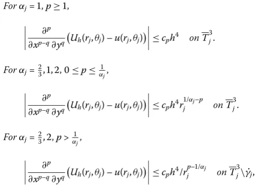
The hexagonal grid version of the block-grid method, which is a difference-analytical method, has been applied for the solution of Laplace’s equation with Dirichlet boundary conditions, in a special type of polygon with corner singularities. It has been justified that in this polygon, when the boundary functions away from the singular corners are from the Hölder classesC4,λ, 0 <

λ

< 1, the uniform error is of orderO(h4_{),his the step size, when the hexagonal grid is applied in the ‘nonsingular’} part of the domain. Moreover, in each of the finite neighborhoods of the singular corners (‘singular’ parts), the approximate solution is defined as a quadrature

approximation of the integral representation of the harmonic function, and the errors of any order derivatives are estimated. Numerical results are presented in order to demonstrate the theoretical results obtained.

Keywords: hexagonal grid; Laplace’s equation; singularity problem; block-grid method

1 Introduction

It is well known that angular singularities arise in many applied problems when the so-lution of Laplace’s equation is considered, and that finite-difference and finite-element methods may become less accurate when singularities are not taken into account. In the last two decades, for the solution of singularity problems, various combined and highly accurate methods have been proposed (see [–], and references therein).

Among these methods the block-grid method (BGM), presented in [–], on polygons with interior anglesαjπ,j= , , . . . ,N, whereαj∈ {_, ,_, }(staircase polygons), requires the finite neighborhood of the singular vertices to be covered by sectors (blocks), and the remaining part of the domain by overlapping rectangles (‘nonsingular’ part). The finite-difference method with square grids is used for the approximate solution in the ‘nonsin-gular’ part, and in the blocks the integral representations of the harmonic function are approximated by the exponentially convergent mid-point quadrature rule (see []). Finally these subsystems are connected together by constructing an appropriate order matching operator. BGM is a highly accurate method not only for the approximation of the solution, but also for the approximation of its derivatives around singular points.

In this paper, the fourth order BGM is extended and justified for the Dirichlet problem of Laplace’s equation on polygons with interior anglesαjπ, where αj∈ {_,_, , }

staircase), by gluing with the matching operator the -point approximation on a hexagonal grid in the ‘nonsingular’ part and the approximation of the integral representations around the singular points (on ‘singular’ parts).

An advantage of using the hexagonal grid version of BGM in this domain is that a highly accurate approximation on the irregular grids is not required as in []. Thus the realization of the total system of algebraic equations becomes simpler. This may not be the case for this type of domain when square or rectangular grids are applied.

Furthermore it is justified that, when the boundary functions on the sides except the adjacent sides of the singular vertices are given inC,λ_{,  <λ< , the proposed hexagonal}

grid version of BGM has an accuracy ofO(h_{),his the mesh step. The same order of}

accuracy is obtained for the -point scheme on a square grid (see [, ]).

Finally in the last section of the paper, numerical experiments are demonstrated to sup-port the theoretical results obtained.

2 Boundary value problem on a special type of polygon

LetDbe an open simply connected polygon,γj,j= , , . . . ,N, be its sides, including the ends, enumerated counterclockwise (γ≡γN,γ≡γN+), and letαjπ,αj∈ {_,_, , }, be the interior angles formed by the sidesγj–andγj. Furthermore, letγ˙j=γj–∩γjbe the jth vertex ofD,γ =_jN_=γjbe the boundary ofD;sis the arclength measured along the boundary ofDin the positive direction, andsjis the value ofsatγ˙j. We denote byrj,θj the polar system of coordinates with poles inγ˙jand the angleθjis taken counterclockwise from the sideγj.

Consider the boundary value problem

u=  onD, ()

u=ϕj onγj,j= , , . . . ,N, ()

where≡∂_/∂x_+∂_/∂y_,ϕ

j,j= , , . . . ,N, are given functions and

ϕj∈C,λ(γj),  <λ< , ≤j≤N. ()

In addition, at the verticesγ˙j, forαj= /, the following conjugation conditions are satis-fied:

ϕ_j(_–p)(sj) =ϕj(p)(sj), p= , . ()

No compatibility conditions are required at the vertices forαj= /. Moreover, it is re-quired that whenαj= /, the boundary functions onγj–andγjare given as algebraic polynomials of the arclengthsmeasured alongγ.

LetE={j:αj= /, ≤j≤N}. We construct two fixed block sectors in the neighbor-hood ofγ˙j,j∈E, denoted byTji=Tj(rji)⊂D,i= , , where  <rj<rj<min{sj+–sj,sj–

sj–},Tj(r) ={(rj,θj) :  <rj<r,  <θj<αjπ}. On the closed sectorT



j,j∈E, we consider the carrier functionQj(rj,θj) in the form given in [], which satisfies the boundary conditions () onγj–∩T



j andγj∩T



We set (see [])

is the kernel of the Poisson integral for a unit circle.

The following lemma acts as a basis for the approximation of the solution around the verticesγ˙jwith angleαjπ,αj= /.

where Vjis the curvilinear part of the boundary of the sector Tj.

For the approximation of problem (), () in the domainD, we apply the hexagonal grid version of the block-grid method (see [–]). The application of this method first of all requires the construction of two more sectorsT_j andT_j, where  <rj<rj<rj. Let hexagonal grid with step sizehl≤h,ha parameter, for the approximation of

Laplace’s equation, and the singular partT_j,j∈E, is approximated by using the harmonic function defined in Lemma ..

() The fourth order matching operator in a hexagonal grid is applied for connecting the subsystems.

() Schwarz’s alternating procedure is used for solving the finite-difference system formed for Laplace’s equation on the parallelograms coveringDT.

Let D_l ⊂ DT, l = , , . . . ,M, be open fixed parallelograms and D ⊂ (M_l=D_l) ∪ (_j∈ET

j)⊂D. We denote byηlthe boundary ofD_l,l= , , . . .M, byVjthe curvilinear part of the boundary of the sector T

j, and lettj= (

M

l=ηl)∩T



j. For the arrangement of the parallelogramsD_l,l= , , . . . ,M, it is required that any pointPlying onηl∩DT, ≤l≤M, or lying onVj∩D, j∈E, falls inside at least on of the parallelogramsD_l(P), ≤l(P)≤M, depending onP, where the distance fromPtoDT∩ηl(P) is not less than

some constantκindependent ofP.

D_lh be the set of grid nodes onD_l,ηh_l be the set of nodes onηl, and letDlh=Dlh∪ηhl.

For the approximation of the solution at the points of the setωh,nwe use the fourth order linear matching operatorSconstructed in [], which can be represented as follows:

S(uh,ϕ) =

Consider the system of difference equations

uh=Suh onD_lh, ()

The solution of this system is the approximation of the solution of problem (), () onDh_∗,n.

Theorem . There is a natural number nsuch that for all n≥nthe system of equations

()-()has a unique solution.

Proof Taking into account the corresponding homogeneous system of system ()-(), the

Now consider the sectorT_j∗=Tj(r∗_j), wherer_j∗= (rj+rj)/,j∈E. Letuhbe the solution

of the system of equations ()-(). The function

Uh(rj,θj) =Qj(rj,θj) +βj 3 Error analysis of the 7-point approximation on the special parallelogram LetD be one of the parallelograms covering the ‘nonsingular’ part of the polygonD de-fined in Section . The boundaries of the parallelogramD are denoted byγ_j, enumer-ated counterclockwise starting from left, including the ends,γ˙_j =γ_j–∩γ_j, j= , , , , denotes the vertices ofD, γ =_j=γ_j, andD =D ∪γ . Furthermoreγ ∩γ =∅, but the vertices γ˙_m with an interior angle ofαmπ=π/ are located either inside ofD, or on the interior of a side γm ofD, ≤m≤N. We define the open parallelogramD as D ={(x,y) :  <y<√a/,d–y/√ <x<e–y/√}. The boundary value problem ()-() is considered onD:

v=  onD, ()

We consider the system of finite-difference equations:

vh=Svh onD_h, ()

Everywhere below we will denote constants which are independent ofhand of the cofac-tors on their right byc,c,c, . . . , generally using the same notation for different constants

for simplicity.

Lemma . Let

ψj(s)∈C,λ

γ_j,  <λ<  ()

and

ψ_j(_–p)(sj) =ψ_j(p)(sj), p= , , ()

be satisfied on the vertices whose interior angles areαjπ=π/,where j= , , , .Then the solution of problem(), ()

v∈C,λD. ()

Proof The closed parallelogramD lies inside the polygonDdefined in Section , and the verticesγ˙_m with an interior angle ofαmπ=π/ are located either inside ofDor on the interior of a sideγmofD, ≤m≤N. Since the boundary functions (), by the definition of the boundary functionsϕjin problem (), () satisfy conditions (), (), from the results

in [], () follows.

LetD_h,k be the set of nodes whose distance from the pointP∈D_h toγ_h is

√

  kh, ≤

k≤a∗, wherea∗= [_√dt

h], [c] denotes the integer part ofc, anddtis the minimum of the half-lengths of the sides of the parallelogram.

Lemma . Let wk_h= const.be the solution of the system of equations wk_h=Swk_h+f_hk on D_h,k,

wk_h=Swk_h on D_h\D_h,k, wk_h=  onγ_h,

and zk

h= const.be the solution of the system of equations z_hk=Szk_h+g_hk on D_h,k,

z_hk=Szk_h on D_h\D_h,k, z_hk=  onγ_h,

where≤k≤a∗.If|fk

h| ≤ghk,then

wk_h≤zk_h, ≤k≤a∗. ()

Proof The proof follows analogously to the proof of the comparison theorem given in

Lemma . Let v be the trace of the solution of problem(), ()on D_h,and vh be the solution of system(), ().If

ψj(s)∈C,λ

γ_j,  <λ< ,j= , , , 

and

ψ_j(_–p)(sj) =ψ_j(p)(sj), p= , ,

on the vertices with an interior angle ofαjπ=π/,j= , , , ,then

max

Dh

|v–vh| ≤ch. ()

Proof Leth=vh–vonDh. Clearly

h=Sh+ (Sv–v) onDh, ()

h=  onγh. ()

LetD_hcontain the set of nodes whose distance from the boundaryγ is

√

h

 , and hence

for (x,y)∈D_h, (x+sH,y+sK)∈D for ≤s≤,H=±h_,±h,K= ,±

√

h

 ,H+K> ,

andD_h=D_h\D_h. Moreover, let

h=h+h. ()

We rewrite problem (), () as

_h=S_h+ (Sv–v) onD_h,

_h=S_h onD_h, ()

_h=  onγ_h

and

_h=S_h onD_h,

_h=S_h+ (Sv–v) onD_h, ()

_h=  onγ_h.

In order to obtain an estimation forSv–vonD_h, we use Taylor’s formula. On the basis of Lemma ., we have

|Sv–v| ≤ch onDh. ()

Since at least two values of

hinShare lying on the boundaryγh, on whichh= , from (), (), and the maximum principle (see []), we obtain

max

Dh

_h≤

maxDh

Hence

max

Dh

_h≤ch, ()

wherec= c.

Next, we consider the estimation of_h. LetD_h,kbe the set of nodes whose distance from the pointP∈D_htoγ_his

√



 kh, ≤k≤a

∗_{, wherea}∗_{= [√}dt

h], [c] denotes the integer part of c, anddtis the minimum of the half-lengths of the sides of the parallelogram. Furthermore, D_h,≡D_handD_h,≡γ_h. Since the vertices withαj=_ of the parallelogramD are never used as a node of the hexagonal grid for the estimation of|Sv–v|onD_h,k, ≤k≤a∗, we use the inequality

max

p+q=

∂_∂_xvp(x_∂,_yyq)

≤cρλ– onD\γm,

for the sixth order derivatives, whereρis the distance from (x,y)∈D toγ_m. Hence, we obtain

|Sv–v| ≤ch/(kh)–λ onDh,k, ≤k≤a∗. ()

Consider a majorant function of the form

Yk=

m ifP∈D_h,m, ≤m≤k,

k ifP∈D_h,m,m>k. ()

HenceYkis a solution of the finite-difference problem

Yk=SYk+μk onDh,k,

Yk=SYk onD_h\D_h,k, ()

Yk=  onγ_h,

where ≤μk≤, ≤k≤a∗.

We represent the solution of system () as the sum of the solution of the following subsystems:

_h,k=S_h_,k+μ_k onD_h,k,

_h,k=S_h_,k onD_h\D_h,k, ()

_h,k=  onγ_h,

where ≤k≤a∗,μ_k=  whenk=  and|μ_k| ≤ch +λ

k–λ whenk= , , . . . ,a∗. By (), (), and Lemma ., it follows that

_h_,k≤c

h+λ

Hence, by taking () and () into consideration, we have

4 Error analysis of the hexagonal block-grid equations Let

h=uh–u, ()

fourth order partial derivatives of the exact solution of problem (), () are bounded onDT. Then estimation () follows from the construction of the operatorS_.

Lemma . There exists a natural number nsuch that for all n≥max{n, [ln+χh–] + }, χ> being a fixed number,

max

j∈E

r_jh≤ch.

Proof The proof follows by analogy to the proof of Lemma . in [].

Theorem . Assume that conditions(), ()hold.Then there exists a natural number n

such that for all n≥max{n, [ln+χh–] + },χ> being a fixed number,

max

Dh_∗,n

|uh–u| ≤ch. ()

Proof Consider an arbitrary parallelogramD_l∗and lett_lh∗_j=Dl∗∩thj. Assume thatthl∗j=∅, zhis the solution of system (), andr_h,r_jh,r_hare defined in the same way as ()-() on

D_l∗, but are zero onDh_∗,n\D_l∗. Hence, V=max

Dh∗,n

|zh|=max

Dl∗

|zh|. ()

We represent the functionzhas

zh=



k=

z_hk, ()

where

z_h=Sz_h+r_h onD_l∗,

z_h=  onηh_l∗_∩γm, z_h=  ont_lh∗_j,

z_h=  onωh,n∩D_l∗,

()

z_h=Sz_h onD_l∗,

z_h=  onηh_l∗_∩γm, z_h=r_jh onth_l∗_j,

z_h=  onωh,n∩D_l∗,

()

z_h=Sz_h onD_l∗,

z_h=  onη_lh∗_∩γm, z_h=  onth_l∗_j,

z_h=r_h onωh,n∩D_l∗

and

z_hk= , k= , ,  onD_∗h,n\D_l∗. () Hence by ()-(),z_hsatisfies the system of equations

z_h=Sz_h onD_l,

As the solution of system (),z_h, is the error function of the finite-difference solution with step sizehl∗≤hof system (), (), by (), the maximum principle and Lemma ., we have

V=max

Dh_∗,n

z_h≤ch. ()

Also, for the solutions of systems () and (), as the operatorShas coefficients which are nonnegative and their sum does not exceed , by the maximum principle, (), Lem-ma ., and LemLem-ma ., we obtain the inequalities

V=max

Now we consider the solution ofv

h. Taking into consideration (), the gluing condition ofD_l,l= , , . . . ,M, andT_j,j∈E, for alln≥max{n, [ln+χh–] + }we have the inequality

For the approximation of (), we consider the following theorem.

number nsuch that for all n≥max{n, [ln+χh–]},χ> being a fixed number,the fol-Proof By taking estimation () into account, the proof follows by analogy to the proof of

Theorem . in [].

5 Numerical results

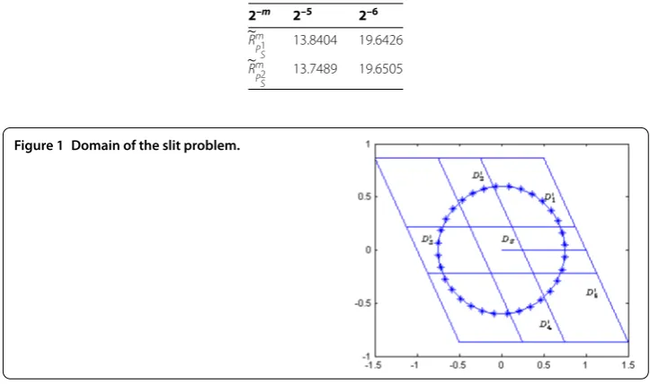
Two examples have been solved in order to test the effectiveness of the proposed method. In Example ., it is assumed that there is a slit in the domainD, thus causing a strong singularity at the origin. The vertexγ˙ containing the singularity has an interior angle of απ= π. The exact solution of this problem is assumed to be known. In Example .,

we consider a problem with two singularities. The vertices which contain the singularities have interior angles ofαjπ=_π,j= , . In this example, the exact solution is not known. After separating the ‘singular’ part in Example ., the remaining part of the domain is covered by  overlapping parallelograms, whereas in Example ., the ‘nonsingular’ part of the domain is covered by only two parallelograms. For the solution of the block-grid equations, Schwarz’s alternating method is used. In each Schwarz iteration the system of equations on the parallelograms are solved by the block Gauss-Seidel method. The carrier function is constructed for each example, taking into consideration the boundary condi-tions given on the adjacent sides of the vertices in the ‘singular’ parts. Furthermore, the derivatives are approximated in the ‘singular’ parts for both of the examples.

The results are provided in Tables -, and Figures -.

Example . Consider the open parallelogramD={(x,y) : – Table 1 Results obtained for the slit problem

(h–1_{, n) u – u}

h_DNS u – uh_DS Rm_DNS Rm_DS

(16, 70) 5.924280×10–5 _5.191270×10–7

Table 2 Results obtained for first derivative of the slit problem

(h–1, n) (16, 70) (32, 70) (64, 110) (128, 130)

(1)

h _DS 7.89831×10–7 9.78871×10–8 4.29502×10–9 2.94108×10–10

Table 3 Results obtained for second derivative of the slit problem

(h–1_{, n) (16, 70) (32, 70) (64, 110) (128, 130)}

_h(2)_DS 3.7119×10–6 9.736×10–7 2.03211×10–8 9.30597×10–10

Table 4 Order of convergence of Example 5.2

2–m ₂–5 ₂–6

Rm

P1_NS 16.257 15.9884

Rm

P2_NS 16.2387 16.0086

Rm P1 S

19.3268 12.7771

Rm P2 S

18.2604 14.0755

Table 5 Order of convergence of derivatives in ‘singular’ parts of Example 5.2

2–m ₂–5 ₂–6

Rm

P_S1 13.8404 19.6426

Rm

P_S2 13.7489 19.6505

Figure 1 Domain of the slit problem.

, , . . . , , be the sides of D, including the ends, enumerated counterclockwise starting from the upper side of the slit (γ≡γ),γ=



j=γj, andγ˙j=γj∩γj–be the vertices ofD.

Let (r,θ)≡(r,θ) be a polar system of coordinates with pole inγ˙, where the angleθ is

taken counterclockwise from the sideγ.

We consider the boundary value problem

u=  onD,

u=ϕj onγj,j= , , . . . , ,

()

where ϕj is the value of the function v(r,θ) = .r/sin_θ + .r/sin_θ + rcosθ + .r_{cosθ+ θ onγ}

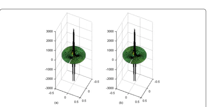
Figure 2 Approximate solution (a) and exact solution (b) of∂_∂u_x, respectively, using polar coordinates.

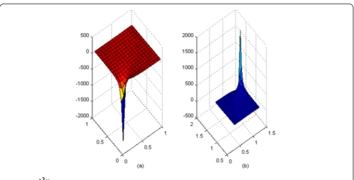
Figure 3 Approximate solution (a) and exact solution (b) of∂2u

∂x2, respectively, using polar coordinates.

Figure 5 ∂2Uh ‘nonsingular’ part, andDS=D\DNSdenote the ‘singular’ part ofD(see Figure ). In Table , the values are obtained in the maximum norm of the difference between the exact and the approximate solutions, for the values ofh= –k_{,k= , , , , andn, which is the number} of quadrature nodes onVj. The order of convergence,RmD=

v–v–mD

v–v_–(m+)D has also been

in-cluded. We also present the error obtained between the derivatives of the exact and the block-grid solutions_h()=r/₍∂u

in Tables  and , respectively. Figures  and  illustrate the shapes of the derivatives ∂u

∂x and∂u

∂x of the approximate (a) and the exact (b) solutions. These figures also demonstrate

the highly accurate approximation of the derivatives.

Example . LetPbe the open parallelogramP={(x,y) :  <y< γj,j= , , , , be the sides ofP, including the ends, enumerated counterclockwise starting from left (γ≡γ,γ≡γ),γ=



j=γj, andγ˙j=γj∩γj–be the vertices ofP. We look at a

problem with two corner singularities at the verticesγ˙andγ˙, whereαjπ=_π,j= , . The two ‘singular’ corners ofPare covered by sectors and these areas are denoted byPi

S, i= , , and two overlapping parallelograms cover the ‘nonsingular’ part of the domain, denoted byPi

NS,i= ,  (see Figure ). We consider the boundary value problem

u=  onP,

u=  onγj,j= , , ()

The carrier functions constructed for each singularity are Q(r,θ) =  – _θπ and

Q(r,θ) = _θ_π. We have checked the accuracy of the obtained approximate resultsuhby

looking at the order of convergence using the formulaRm_P =u–m–u–m+P

u_–m––u–mP, which

corre-sponds to _{, for the pairs (h,n) = (}–_{, ), (}–_{, ), (}–_{, ), (}–_{, ). The results are}

presented in Table . Moreover,∂u

∂x has been approximated in the ‘singular’ part, whereu

is the unknown exact solution of problem (). The results are presented in Table  and illustrated further in Figure .

6 Conclusion

A fourth order square and hexagonal grid version of the block-grid method, for the so-lution of the boundary value problem of Laplace’s equation on staircase polygons, with interior angles αj∈ {_, ,_, }, is extended for the polygons with interior angles αjπ,

αj∈ {_,_, , }, by constructing and justifying the block-hexagonal grid method. Moreover, the smoothness requirement on the boundary functions away from the singular vertices (outside of the ‘singular’ parts) is lowered down from the Hölder classesC,λ_{,  <λ< ,}

as in [], toC,λ_{,  <λ< , which was proved for the -point scheme on square grids (see}

[, ]).

The proposed version of the BGM can be applied for the mixed boundary value problem of Laplace’s equation on the above mentioned polygons. Furthermore, by this method any order derivatives of the solution can be highly approximated on the ‘singular’ parts, which are difficult to obtain in other numerical methods.

This method can also be used for the solution of the biharmonic equation by represent-ing the problem with two problems for the Laplace and Poisson equations.

Competing interests

The authors declare that they have no competing interests.

Authors’ contributions

All authors contributed equally to the writing of this paper. All authors read and approved the final manuscript.

Received: 1 December 2014 Accepted: 9 February 2015 References

1. Li, ZC: A nonconforming combined method for solving Laplace’s boundary value problems with singularities. Numer. Math.49(5), 475-497 (1986)

2. Li, ZC: Combined Methods for Elliptic Problems with Singularities, Interfaces and Infinities. Kluwer Academic, Dordrecht (1998)

3. Olson, LG, Georgiou, GC, Schultz, WW: An efficient finite element method for treating singularities in Laplace’s equation. J. Comput. Phys.96(2), 391-410 (1991)

4. Xenophontos, C, Elliotis, M, Georgiou, G: A singular function boundary integral method for Laplacian problems with boundary singularities. SIAM J. Sci. Comput.28(2), 517-532 (2006)

5. Georgiou, GC, Smyrlis, YS, Olson, L: A singular function boundary integral method for the Laplace equation. Commun. Numer. Methods Eng.12(2), 127-134 (1996)

6. Dosiyev, AA: A block-grid method of increased accuracy for solving Dirichlet’s problem for Laplace’s equation on polygons. Comput. Math. Math. Phys.34(5), 591-604 (1994)

7. Dosiyev, AA: The high accurate block-grid method for solving Laplace’s boundary value problem with singularities. SIAM J. Numer. Anal.42(1), 153-178 (2004)

8. Dosiyev, AA, Celiker, E: Approximation on the hexagonal grid of the Dirichlet problem for Laplace’s equation. Bound. Value Probl.2014, 73 (2014)

9. Volkov, EA: An exponentially converging method for solving Laplace’s equation on polygons. Math. USSR Sb.37(3), 295-325 (1980)

10. Dosiyev, AA: On the maximum error in the solution of Laplace equation by finite difference method. Int. J. Pure Appl. Math.7, 229-242 (2003)

11. Dosiyev, AA, Buranay, SC: A fourth order accurate difference-analytical method for solving Laplace’s boundary value problem with singularities. In: Tas, K, Machado, JAT, Baleanu, D (eds.) Mathematical Methods in Engineering, pp. 167-176. Springer, Berlin (2007)

13. Samarskii, AA: The Theory of Difference Schemes. Dekker, New York (2001)