Lagged diffusivity method for the solution of nonlinear diffusion convection problems with finite differences

R E S E A R C H

Open Access

Lagged diffusivity method for the solution of

nonlinear diffusion convection problems with

finite differences

Emanuele Galligani

Correspondence: emanuele. [email protected]

Dipartimento di Matematica Pura e Applicata_“G.Vitali_”, Università degli Studi di Modena e Reggio Emilia, Via Campi 213/b, I-41125 Modena, Italy

Abstract

This article concerns with the analysis of an iterative procedure for the solution of a nonlinear nonstationary diffusion convection equation in a two-dimensional bounded domain supplemented by Dirichlet boundary conditions. This procedure, denoted Lagged Diffusivity method, computes the solution by lagging the diffusion term. A model problem is considered and a finite difference discretization for that model is described. Furthermore, properties of the finite difference operator are proved. Then, a sufficient condition for the convergence of the Lagged Diffusivity method is given. At each stage of the iterative procedure, a linear system has to be solved and the Arithmetic Mean method is used. Numerical experiments show the efficiency, for different test functions, of the Lagged Diffusivity method combined with the Arithmetic Mean method as inner solver. Better results are obtained when the convection term increases.

1 Statement of the problem

Consider as model problem the nonlinear diffusion convection equation

∂u

∂t = div(σ∇u)− ˜v· ∇u−αu+s, (1)

whereu=u(x, y, t) is the density function at the point (x, y) at the timetof a diffu-sion medium R, s= s(x, y, u) > 0 is the diffusion coefficient or diffusivity and is dependent on the solutionu,a =a(x, y)≥0 is the absorption term, v˜=v(x,˜ y,t,u) is the velocity vector and the source terms(x, y, t) is a real valued sufficiently smooth function.

Equation (1) can be supplemented by the initial condition (t= 0)

u(x,y, 0) =U0(x,y), (2)

in the closure _R¯ ofRand by Dirichlet boundary condition on the contour∂RofRof the form

u(x,y,t) =U1(x,y,t). (3)

In the following, we supposeRto be a rectangular domain with boundary∂Rand we assume that the functionss,a, andssatisfy the“smoothness” conditions:

(i) the function s=s(u) is continuous inu;the functions a(x, y) and s(x, y, t) are continuous inx, y and inx, y, trespectively;

(ii) there exist two positive constants sminandsmaxsuch that

0< σmin≤σ(u)≤σmax,

uniformly inu; in addition,a(x, y)≥amin≥0;

(iii) for fixed (x, y)ÎR, the functions(u) satisfies Lipschitz condition inuwith con-stantΓ(uniformly in x, y),Γ> 0.

Here, the vector v˜= (v˜1,v˜2)T is assumed to be constant.

The nonlinearity introduced by the u-dependence of the coefficient s(u) requires that, in general, the solution of equation (1) be approximated by numerical methods.

We superimpose on R∪∂Ra grid of pointsRh∪ ∂Rh; the set of the internal points Rhof the grid are the mesh points (xi,yj), fori= 1,...,Nandj= 1,...,M, with uniform mesh size halongx andy directions, respectively, i.e.,x_i+1=xi +handyj+1=yj+h for i= 0,...,N, j= 0,...,M.

Thus, at the mesh points of R∪∂R, (x_i,y_j), fori= 0,..., N+ 1, j= 0,..., M + 1, the solution u(x_i, y_j,t) is approximated by a grid function u_ij(t) defined onR_h∪∂R_h and satisfying the boundary condition (3) on∂R_hfort> 0 and the initial condition (2) on Rh∪∂Rhfor t= 0.

By ordering in a row lexicographic order the mesh pointsP_l= (x_i,y_j) (i.e.,l= (j- 1)⋅ N+iwithj= 1,..., M, andi= 1,..., N), we can write the vectoru(t) of componentsu_ij (t) and approximate the right-hand side of (1) by

A(u(t))u(t) +b(u(t)) +s(t), (4)

where the matrixA(u(t)) is of order μ=M×Nand has the block tridiagonal form; the M diagonal blocks are tridiagonal matrices of order Nand the M - 1 sub- and super-diagonal blocks are diagonal matrices of orderN.

The five nonzero elements ofA(u(t)) corresponding touij-1(t), ui-1j(t),uij(t),ui+1j(t) and uij+1(t) respectively, are

{(Bij+B˜ij), (Lij+L˜ij),−(Dij+Dˆij), (Rij+R˜ij), (Tij+T˜ij)},

where

Lij≡Lij(u(t)) =

1 h2σ

uij(t) +ui−1j(t)

2

,

Bij≡Bij(u(t)) =

1 h2σ

uij(t) +uij−1(t)

2

,

Rij≡Rij(u(t)) =

1 h2σ

ui+1j(t) +uij(t)

2

,

Tij≡Tij(u(t)) =

1 h2σ

uij+1(t) +uij(t)

2

,

˜ Lij= ˜

v1

2h,B˜ij= ˜ v2

2h, ˜

Rij=−˜

v1

2h,T˜ij=− ˜ v2

2h, Dij≡Dij(u(t)) =Bij+Lij+Rij+Tij,Dˆij=α(xi,yj).

The matrixA(u(t)) is an irreducible matrix [[1], p. 18]. Providing that the mesh spacinghis sufficiently small, i.e.,

h<min

2σmin v_˜1

,2σmin ˜ v2

, (6)

the matrixA(u(t)) is strictly (a(x, y) > 0) or irreducibly (a(x, y) = 0) diagonally domi-nant ([[1], p. 23]) and has negative diagonal elements, all(u(t)) < 0 (l= 1, ..., μ) and nonnegative off diagonal elementsalp(u(t))≥0,l ≠p, withl, p= 1, ..., μ; therefore, -A (u(t)) is an M-matrix [[1], p. 91].

In the case of diffusion equation(˜v=0), the matrixA(u(t)) is also symmetric; then -A(u(t)) is a Stieltjes matrix and is symmetric positive definite [[1], p. 91].

The vector b(u(t)) in (4) is obtained imposing Dirichlet boundary conditions (3) and it depends on the function U1(x_i, y_j, t) at points (x_i,y_j) of ∂R and itslth component depends on the lth component of the solutionu(t) for the mesh pointP_lofRwhich is neighbor of points of ∂R.

The vector s(t) in (4) has componentssl(t) =s(xi, yj,t) fori= 1,..., N, j= 1,...,M and l= (j- 1)N+i.

We can apply a step-by-step method to the initial value problem ofμequations

du(t)

dt =A(u(t))u(t) +b(u(t)) +s(t),

with the initial condition (2), u(xi, yj, 0) =U0(xi,yj), and computes the approximation un+1

tou(tn+1) using the approximate solutionun at the time leveltn, with tn=nΔt and Δtthe time step.

Indicating sn=s(tn), forn= 0,1,..., the well-knownθ-method (see, e.g., [2]) is written

un+1_−un

t =θ(A(un+1)un+1+b(un+1) +sn+1) + (1−θ)(A(un)un+b(un) +sn),

whereθis a real parameter such that 0≤θ≤1; for anyθ≠0, the method is implicit. Iis theμ×μidentity matrix.

Thus, at each time level n= 0, 1,..., the vectorun+1Îℝμis the solution of the non-linear system,

F(u)≡(I−tθA(u))u−tθb(u)−w=0. (7)

The vectorwÎℝμis given by

w≡wn= (I+t(1−θ)A(un))un+t(1−θ)b(un) +t(θsn+1+ (1−θ)sn).

We setτ =Δtθ.

We can introduce an iterative method of Lagged Diffusivity, computing the new iter-ate u(k+1) keeping the diffusivity term at the previous iterationk. That is, since the matrix I-τ A(u) is nonsingular for alluÎ ℝμthen u(k+1)is the solution of the linear system

such that the residual

r(k+1)= (I−τA(u(k)))u(k+1)−w−τb(u(k)),

satisfies the stopping condition

r(k+1)≤εk+1,

where εk is a given tolerance such that εk® 0 when k® ∞ and∥⋅∥ indicates the Euclidean norm. The initial iterate u(0)of this Lagged Diffusivity procedure can be set equal toun.

2 Uniform monotonicity and a convergence result

In this section, we consider the nonlinear system F(u) =0in (7) and we prove thatF (u) is continuously and uniformly monotone and then F(u) = 0has a unique solution. Moreover, we prove that the sequence {u(k)} generated by the Lagged Diffusivity pro-cedure is convergent to the solution. Before this, we have to prove three lemmas on some properties of finite difference operators.

In the following, we may consider the matrixA(u) as

A(u) =A(u) +ˆ A˜+D,ˆ

where A(u)ˆ and A˜ are the block tridiagonal matrices whose row elements are {Bij,

Lij, -Dij, Rij, Tij} and { ˜Bij,L˜ij,R˜ij,T˜ij}, respectively, while the matrix Dˆ is a diagonal matrix whose diagonal entries are {− ˆDij}. Furthermore, we denote

ˆ

A(u) =Aˆx(u) +Aˆy(u),

where Aˆx_{(u) is the block diagonal matrix whose row elements are} {Lij,−Dxij,Rij}

with Dx_ij=Lij+Rij, and Aˆy(u) is the block tridiagonal matrix whose row elements are

{Bij,−Dyij,Tij} with Dyij=Bij+Tij. Analogously, we can define b(u) = bx(u) + by(u) wherebx(u) contains the contributions of U1(x0, yj,t) andU1(xN+1, yj,t) forj= 1, ...,M and by(u) contains the contributions ofU1(xi,y0,t) andU1(xi,yM+1,t) fori= 1,...,N.

For the sake of clarity, we setuij≡ uij(t) and vij ≡vij(t), (i= 0,...,N+ 1,j= 0,...,M + 1), the grid functions defined onR_h∪∂R_hand satisfying the Dirichlet boundary condi-tion on∂R_hfort> 0.

For grid functions {u_ij} and {v_ij} of this type, the discretel2 (R_h) inner product and norm are defined by the formulas

<u,v>=h2

N

i=1 M

j=1

uijvij,

uh= (h2 N

i=1 M

j=1 uij

2

)1/2= (<u,u>)1/2,

respectively

constantsrandb, both independent ofh, such that

uh≤ρ (8)

_∇xuij≤β, ∇yuij≤β. (9)

Here,∇xuijand ∇yuijindicates the backward difference quotients

∇xuij=

uij−ui−1j

h , ∇yuij=

uij−uij−1

h . (10)

Before to prove the main result, we summarize in three lemmas on some properties of finite difference operators.

Here, for a grid function {u_ij}, we denote

ui±1/2j=

ui±1j+uij

2 , uij±1/2=

uij±1+uij

2 .

Lemma 1. Let {u_ij}, {v_ij}, {z_ij} be three grid functions defined at the mesh points (x_i, yj) of a gridRh∪∂Rh,i = 0,...,N+ 1,j= 0,...,M +1 which are equal to the prescribed functionU1 (x_i, y_j,t) at the point (x_i,y_j) of∂R_handt> 0; then

<− ˆA(z)u−b(z),v>=<− ˆAx(z)u−bx(z),v>+<− ˆAy(z)u−by(z),v>,

where

<− ˆAx(z)u−bx(z),v>=

M

j=1

σ(z1/2j)(u1j−u0j)v1j+

+

N

i=2

σ(zi−1/2j)(uij−ui−1j)(vij−vi−1j)+

+σ(zN+1/2j)(uNj−uN+1j)vNj

,

(11)

<− ˆAy(z)u−by(z),v>=

M

i=1

σ(zi1/2)(ui1−ui0)vi1+

+

M

j=2

σ(zij−1/2)(uij−uij−1)(vij−vij−1)+

+σ(ziM+1/2)(uiM−uiM+1)vMj

.

(12)

Proof. Formulae (11) and (12) follow immediately from the definition of the coeffi-cients in (5).

Lemma 2. Let {u_ij} and {v_ij} be two grid functions defined at the mesh points (x_i,y_j) of the grid R_h∪ ∂R_h, i= 0,..., N+ 1,j = 0,..., M+ 1 such that, at the point (x_i,y_j) of ∂Rhandt> 0, the grid function {uij} is equal to the prescribed functionU1(xi,yj,t) and the grid function {v_ij} is equal to the null function, respectively.

<− ˆA(u)v,v>=h2

From the definition of backward difference quotients (10), we have formula (13). Lemma 3. Let {u_ij}, {v_ij} and {˜vij} be three grid functions of B such that, at the points (x_i,y_j) of the boundary∂R_hthey are equal to the prescribed functionU1(x_i,y_j,t) (t> 0).

Then, we have the following expression for the discretel2(R_h) inner product

Writing the backward difference quotients (10) for the functions v˜ij and uij− ˜vij and

Since the property of Lipschitz continuity on the function swith Lipschitz constant

Γ (property (iii)), we have for an arbitrary positive number j, we have

M

Then, we have the result (14).

As a consequence of Lemmas 1, 2, and 3, we prove the result of the uniform mono-tonicity of the mapping F(u); thus the nonlinear system (7) has a unique solution in

B. Proof. We show that the mappingF(u) is continuous and uniformly monotone, i.e., there exists a positive scalargsuch that

We separately examine the terms

<− ˆA(u)(u−v),u−v>,<(− ˆD+1

τI)(u−v),u−v> and

<(− ˆA(u) +A(v))vˆ −b(u) +b(v),u−v>.

Lemma 2 withu-vinstead ofvand the assumption (ii) on the uniform lower bound-edness ofsrespect to the variableupermit to write

<− ˆA(u)(u−v),u−v>≥h2σmin

Then, collecting the last three inequalities we obtain

1

When condition (15) holds, then the mapping F(u) is uniformly monotone on _B where the constantgin (16) is

γ =τ

Now, we can state a result for the convergence of the Lagged Diffusivity method where the vector u(k+1)is the approximate solution of the linear system

such that the residual

r(k+1)= (I−τA(u(k)))u(k+1)−w−τb(u(k)),

satisfies the stopping condition

r(k+1)≤εk+1, (18)

whereεkis a given tolerance such thatεk®0 whenk® ∞.

Thus, the iterateu(k+1)is the solution of the system (7) whose diffusivity termsinA (u) andb(u) depends on the iterateu(k)and the inhomogeneous term now depends by u(k+1)

.

We suppose that the grid functions {u(k)_ij },k= 0, 1, ..., are belonging to the set B. In

particular, the backward difference quotients of each grid function {u(k)_ij } are bounded.

Since this bound depends on the inhomogeneous term, we have that there exist two constantsb> 0 andb0> 0 such that

∇xu

(k)

ij ≤ ˜βk and ∇yu (k)

ij ≤ ˜βk, (19)

with _β˜k=β+εkβ0. (Formula (19) replaces formula (9).)

Theorem 4. Letu∗∈Bbe the solution of the nonlinear systemF(u) =0in (7). Letu (k+1)

be the solution of the linear system in (17) with condition (18). If condition (15) is satisfied, and, in particular

αmin+

1 τ >

σmin

h2 , (20)

then, the sequence {u(k)} converges tou*.

Proof. The solutionu∗ ∈Bof (7) satisfies the equation

u∗−τA(u∗)u∗−w−τb(u∗) =0, (21)

and the iterateu(k+1) satisfies the equation

u(k+1)−τA(u(k))u(k+1)−w−τb(u(k)) =r(k+1). (22)

Subtracting (22) from (21), we obtain

−A(u∗)u∗+A(u(k))u(k+1)+1 τu∗−

1

τu(k+1)−b(u∗) +b(u(k)) =− 1 τr(k+1).

Taking into account of the identity

−A(u)u+A(w)v=−A(u)(u−v) + (−A(u) +A(w))v,

for all u, vand wbelonging to B, we can write

−A(u∗) +1

τI

(u∗−u(k+1)) + (−A(u∗) +A(u(k)))u(k+1)−b(u∗) +b(u(k)) = 1

Thus, we have

and then, we can write

<−1_τr(k+1),u∗−u(k+1)> ≥

≥<− ˆA(u∗)(u∗−u(k+1)),u∗−u(k+1)>+<(− ˆD+1

τI)(u∗−u(k+1)),u∗−u(k+1)>−

−<(− ˆA(u∗) +Aˆ(u(k)))u(k+1)−b(u∗) +b(u(k)),u∗−u(k+1)>.

From Lemmas 2 and 3 we obtain

<−1

Keeping into account of the stopping condition (18) we can write

1

Since jis an arbitrary positive number, we can choose jsuch that in (23)

σmin−

˜ βk+1φ

that is

φ = 2_˜σmin βk+1

.

Thus, from (23) and (24) we have

1

Since the grid function {u(k+1)_ij } belongs to _B, it then satisfies the inequality (8) and

so we have

We assume that condition (15) holds. Then, keeping into account of the expression of _β˜k, we have the inequality

Therefore, the sequence {u(k)} of approximate solutions of the Lagged Diffusivity method converges to the solution u* of the system (7).

3 Numerical experiments

In this section, we consider a numerical experimentation of the Lagged Diffusivity method for the solution of the nonlinear system generated by theθ-method applied on the model problem (1) in a rectangular domain with Dirichlet boundary conditions. Indeed we solve with the Lagged Diffusivity procedure the nonlinear system

The Lagged Diffusivity procedure is an efficient and robust method, even if only line-arly convergent, for solving the digital image restoration problem using diffusive filters. One of the most used diffusive filter is defined (in equation (1) with(˜v=0)) by a dif-fusivitys(u) chosen as a rapidly decreasing function of the gradient magnitude |∇u|2. Specifically, s(s) : [0, ∞) ® (0, ∞) is a decreasing function satisfying s(0) = 1 and lims®∞s(s) = 0 ands= |∇u|2= (∂u/∂x)2+ (∂u/∂y)2.

Due to the presence of this term s(u), the operator div(s∇u) is highly nonlinear and, when linearized by lagging the diffusivitys, it has highly varying coefficients [4-8].

Often happens in real images that |∇u| = 0. This makes necessary the use of numeri-cal regularization, consisting in replacing the term |∇u| by (|∇u|2 +b)1/2for a“small enough” positive artificial parameter b. Due to the presence of the highly nonlinear operator div(s∇u), Newton’s method for solving the nonlinear system (7) does not work satisfactory, in the sense that its domain of convergence is very small.

These diffusion problems for image restoration are also solved using operator split-ting methods (e.g., [9-11]). Operator splitsplit-ting is a powerful concept used in Computa-tional Mathematics for the design of effective numerical methods. These splitting methods are essentially based on certain special relaxation processes which allow one, to reduce the complicated problem into a sequence of simpler problems which can be effectively solved with a computer.

At present, there exists a lot of interest in the applications of operator splitting methods to problems of Financial Mathematics, and, in particular, to diffusion convec-tion equaconvec-tions with mixed derivatives terms (e.g., [12-14]).

Operator splitting is also a very common tool for solving nonlinear evolution equa-tions which include hyperbolic conservation laws and degenerate diffusion convection equations with nonsmooth solutions. In these evolution equations, the convection dominates diffusion (e.g., [15-19]).

An alternative case has been considered in our computational experiments. Indeed, we consider diffusion convection problems which are of diffusion dominated nature, as those concerning the groundwater transport of a contaminant in an aquifer or the con-trol of heating processes of industrial kilns.

The convergence of the “outer”iteration {u(k)} to u* of the Lagged Diffusivity proce-dure involves solution for an unknown vectoruof the matrix equation (17). This lin-ear system may be solved by an operator splitting method. The effect of this “inner” iteration on convergence of the “outer” iteration tou* must be analyzed in order to define a good strategy for the convergence of the Lagged Diffusivity procedure. Indeed, a significant reduction in total effort can often be achieved by proper coordination of inner and outer iteration.

In the experiments, the vector solution u* is prefixed and is composed by the values of prescribed functionsu(x, y, t) defined on [a, b] × [a, b] × [0, ∞). In all the experi-ments, we have a = 0 andb = 1. We choose different solution functions where the time valuetis set equal to 1:

u1 :u(x,y,t) =xyt,

u2 :u(x,y,t) =

3

i=1

15e−8((x−ξi)2+(y−ηi)2)t_,

u3 :u(x,y,t) = (x+y)t,

For the functionu2, we haveξ1 =h1= 0.2,ξ2= 0.2,h2= 0.8 andξ3 =h3= 0.8. The chosen functionss(u) are:

σ1 :σ(u) = 0.01 + 0.5u, σ2 :σ(u) = 0.01 + 0.5u2, σ3 :σ(u) = 100

1 + 500u.

The vectorwis computed as

w≡w∗= (I−τA(u∗))u∗−b(u∗),

where the matrixA(u*) and the vectorb(u*) have elements as in formula (5) withN =Mand a(x, y) = 0. We setθ= 1 andΔt= 10-3orΔt= 10-4;τ=θΔt. Here, the con-dition (20) holds.

At each iteration kof the Lagged Diffusivity procedure, we have to solve the linear system of orderμ=N×N:

(I−τA(u(k)))u=w∗+b(u(k)).

We consider the case that the coefficient matrix is an M-matrix(˜v= 0).

In these experiments, the iterative method of the Arithmetic Mean is used as linear solver in the form introduced in [20]. This method is convergent when the coefficient matrix is a nonsingular M-matrix. This form of the Arithmetic Mean method is a var-iant of the Alterating Group Explicit (AGE) decomposition introduced by Evans (e.g., see [21-23]). The effectiveness of the Arithmetic Mean method, even on parallel archi-tectures, is highlighted in [20,24-27]. Some recent papers on the Arithmetic Mean method on linear systems are in [28-31].

We callu(k+1)the solution of the linear system above computed withjkiterations of the Arithmetic Mean solver where the inner residual

r(k+1)= (I−τA(u(k)))u(k+1)−w∗−b(u(k)),

satisfies the condition

r(k+1)≤εk+1,

withε1= 0.1∥F(u(0))∥and

εk+1= 0.5εk. (26)

The vector F(u(0)) = (I- τA(u(0)))u(0)-w* -b(u(0)) is the initial outer residual and its Euclidean norm is calledres0.

The initial vector u(0)is taken as the null vector (u(0)=0) or as the vectorewhich is the vector with all the components equal to 1 (u(0)=e).

The Lagged Diffusivity procedure has been implemented in a Fortran code with machine precision 2.2 × 10-16and stops when

εk+1≤ε, (27)

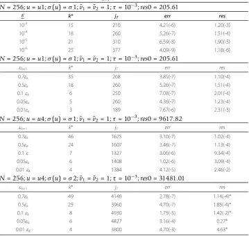
An experiment evaluates the effectiveness of the Lagged Diffusivity method for differ-ent values of ε; another experiment shows the behavior of the method for different choices of εk+1respect to the one in (26) with ε= 10−4.

We call k* the iteration of the Lagged Diffusivity procedure for which condition (27) is satisfied.

In the tables, we report the number of iterationsk*, the total number of iterations of the Arithmetic Mean method jT, the discrete l2(Rh) norm of the error,

err=u∗−u(k∗)

h, the Euclidean norm of the outer residual

res=F(u(k∗))=(I−τA(u(k∗)))u(k∗)−w∗−b(u(k∗)),

and res0.

The symbol * close to the value ofresindicates that the behavior of the norm of the outer residual (∥F(u(k))∥) is not monotone decreasing. In addition, _σ¯∗ is an approxima-tion ofsmax.

Furthermore, in the tables, writing 5.26(-7) means 5.26 × 10-7.

From the numerical experiments, we can drawn the below conclusions (See Tables 1, 2 and 3).

•We observe that, sinceεk+1decreases, for kincreasing, as (26) and the Lagged Diffusivity method stops at the iterationk* when the criterium for εk∗+1 in (27) is satisfied, we have

εk∗+1=

1 2εk∗=

1

22εk∗−1=· · ·=

1 2k∗ε1≤ε,

where we setε1= 0.1∥F(u(0))∥. Then

k∗ >log₂

_ε 1

ε

.

In the experiments, we obtain

k∗ =

log₂

ε1

ε

.

• We observe that in all the experiments with the rule (26) the outer residual F(u(k∗))has the same order of ε with an error in the discrete l2(Rh) norm of

order of hε.

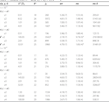
•About the initial vectors, we can say that, generally, the null vector is a good choice, in terms of total number of inner iterations, fors(u) =s1 ands(u) =s2; while for the functionsu(x, y, t) ands(u) =s3 we have better results whenu(0)=e. A detection of that the null vector is not a good initial vector for the problems withs(u) =s3, is the number of inner iterations at the first outer iteration. Indeed, for the functionsu2, u3, and u4, most of the inner iterations happen at the first iteration,k= 1; for instance, in Table 1 whens(u) =s3 andτ = 10-4, atk= 1, for u2 we have 1,484 inner iterations on the total number 1,534, foru3 we have 1,421 inner iterations on the total number 1,515, for u4 we have 1,407 inner iterations on the total number 1,986.

•When the behavior of the norm of the outer residual F(u(k)) is not monotone decreasing (i.e.,s(u) = s2,u(x, y, t) =u2,u4, τ= 10-3) we can have a large total number of inner iterations at an outer iteration. We suggest to change the initial vector to obtain a monotone decreasing of the norm of the outer residual that implies a reduction of the total number of inner iterations. Changing the initial vectoru(0), the rows marked with“✔”in Table 1 become the results of Table 4. •From Table 1, we observe that the Arithmetic Mean method gives better perfor-mances when the ratio σ∗/˜v1(˜v1=v˜2) is small, that is the coefficient matrix of the inner linear system is strongly asymmetric (see [24]).

Table 1 Results withN= 256, v˜1=v˜2= 1,u(0)= 0

u(x, y, t) σ¯∗/˜v1 k* jT err res res 0 τ= 10-3

s(u) =s1

u1 0.51 18 260 5.26(-7) 1.51(-4) 205.61

u2 8.52 26 5972 4.81(-7) 1.48(-4) 51451.65

u3 1.01 20 585 7.00(-7) 1.97(-4) 1041.69

u4 4.01 24 1607 3.46(-7) 1.13(-4) 9617.82

s(u) =s2

u1 0.51 17 196 5.96(-7) 1.80(-4) 123.15

✔u2 145.03 29 35427 2.19(-7) 9.73(-5)* 276108.92

u3 2.01 20 899 5.59(-7) 1.71(-4) 898.18

✔u4 32.01 25 3960 4.70(-7) 1.85(-4)* 31481.01

τ= 10-4

s(u) =s1

u1 0.51 17 33 4.22(-7) 1.12(-4) 89.44

u2 8.52 23 676 5.40(-7) 1.45(-4) 6203.62

u3 1.01 19 70 3.75(-7) 9.94(-5) 304.43

u4 4.01 21 216 3.80(-7) 1.10(-4) 1170.79

s(u) =s2

u1 0.51 17 30 3.54(-7) 9.63(-5) 86.61

u2 145.03 25 7160 4.65(-7) 1.55(-4) 28054.93

u3 2.01 19 115 4.00(-7) 1.10(-4) 297.76

u4 32.01 22 852 4.43(-7) 1.53(-4) 3266.07

s(u)=s3

u2 1.50 22 1534 4.19(-7) 1.30(-4) 3061.65

u3 100.00 19 1515 3.16(-7) 1.10(-4) 297.96

•A very general conclusion is that, at each time step t_n, the Lagged Diffusivity method (17)-(18)-(26)-(27) allows to obtain an approximate solution of the non-linear system (7) with sufficiently high accuracy and low computational complexity, when the initial vectoru(0)has been chosen properly.

Remark. Given the exact solution u(x, y, t) of equations (1), (3) at timet=t_n+1(for example, tn+1= 1), in the above numerical experiments, we have considered in system (7) the“source” vectorwasw≡ w* = (I-τA(u*))u* -b(u*) withu* = {u(xi,yj,tn+1)}.

With this definition of w, it has been possible to obtain, for our test problems, the behavior of the error associated with the numerical computation of the solution of (7), i.e., an indication of the accuracy on the solution of the nonlinear equations (7). We have denoted this error by err.

In order to analyze the behavior of the effective one-step error(in the discretel2(R_h) norm) of the θ-method, denoted byEstep, we must consider in system (7) the“source” vectorwas

w≡wn=I+t(1−θ)A(un)un+t(1−θ)b(un) +t(θsn+1+ (1−θ)sn)

withun= {u(x_i,y_j,t_n)} andt_n=t_n+1-Δt.

From Table 5, we observe that the values of Estep are comparable with those of err, with the exception of the test problemss(u) =s1,s2,u(x, y, t) =u2 forτ= 10-3, 10-4,

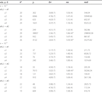
Table 2 Results withN= 256, v˜1=v˜2= 1,u(0)=e

u(x, y, t) k* jT Err res res0

τ= 10-3

s(u) =s1

u1 20 302 3.69(-7) 1.03(-4) 546.04

u2 26 6066 4.76(-7) 1.47(-4) 50940.66

u3 20 633 4.63(-7) 1.31(-4) 692.97

u4 24 1631 3.37(-7) 1.10(-4) 9323.23

s(u) =s2

u1 19 249 4.51(-7) 1.32(-4) 362.86

u2 29 38837 2.36(-7) 1.06(-4)* 298830.38

u3 20 932 5.45(-7) 1.67(-4) 881.87

u4 26 4122 2.63(-7) 1.03(-4)* 35275.82

τ= 10-4

s(u) =s1

u1 18 37 5.17(-7) 1.34(-4) 211.75

u2 23 737 5.23(-7) 1.40(-4) 6026.72

u3 18 76 3.73(-7) 9.89(-5) 132.60

u4 21 240 3.46(-7) 1.00(-4) 1074.69

s(u) =s2

u1 18 33 4.50(-7) 1.19(-4) 205.39

u2 25 7615 5.02(-7) 1.68(-4)* 30266.34

u3 18 121 3.82(-7) 1.05(-4) 144.41

u4 22 910 4.89(-7) 1.69(-4) 3611.96

s(u) =s3

u2 22 48 3.98(-7) 1.24(-4) 2825.73

u3 17 102 4.76(-7) 1.66(-4) 113.34

where the discrepancy between errandEstepdepends on the fact that the matrixA(u) is ill conditioned because the Lipschitz constant is large.

Furthermore, the global error for solving the problem (1)-(2)-(3) with theθ-method combined with the Lagged Diffusivity procedure is computed for the cases

c1 :θ = 1, ux,y,t=u2,σ(u) =σ1, c2 :θ = 0.5,u(x,y,t) =u2,σ(u) =σ1, c3 :θ = 1, u(x,y,t) =u4,σ(u) =σ1, c4 :θ = 0.5,u(x,y,t) =u4,σ(u) =σ1,

and it is denoted withE(c1),E(c2),E(c3), andE(c4).

The behavior of this global error, step-by-step, from 1 ≤t ≤ 1.2 and Δt= 10-3 is highlighted in Figure 1; the numerical results are seen to be largely in keeping with the theory.

Table 3 Results for different ε andε_k+1(u(0)=0)

N= 256;u=u1;σ(u) =σ1;v˜1=v˜2= 1;τ = 10−3;res0 = 205.61

ε k* jT err res

10-3 _{15 210 4.21(-6) 1.20(-3)}

10-4 _{18 260 5.26(-7) 1.51(-4)}

10-5 _{21 310 6.59(-8) 1.90(-5)}

10-6 25 377 4.09(-9) 1.18(-6)

N= 256;u=u1;σ(u) =σ1;v˜1=v˜2= 1;τ = 10−3;res0 = 205.61

εk+1 k* jT err res

0.7_εk 35 268 3.85(-7) 1.10(-4)

0.5εk 18 260 5.26(-7) 1.51(-4)

0.1εk 6 250 7.08(-7) 2.01(-4)

0.05εk 5 260 4.36(-7) 1.23(-4)

0.01εk 3 189 7.67(-6) 2.31(-3)

N= 256;u=u4;σ(u) =σ1;˜v1=˜v2= 1;τ = 10−3;res0 = 9617.82

εk+1 k* jT err res

0.7εk 46 1625 3.10(-7) 1.02(-4)

0.5εk 24 1607 3.46(-7) 1.13(-4)

0.1ε 7 1327 3.06(-6) 9.34(-4)

0.05εk 6 1408 1.02(-6) 3.09(-4)

0.01_εk 4 1384 4.12(-5) 2.46(-2)

N= 256;u=u4;σ(u) =σ2;v˜1=v˜2= 1;τ = 10−3;res0 = 31481.01

εk+1 k* jT err res

0.7εk 49 4146 2.78(-7) 1.14(-4)*

0.5εk 25 3960 4.70(-7) 1.85(-4)*

0.1εk 8 4930 1.75(-5) 1.42(-2)*

0.05εk 6 4827 3.16(-4) 0.27*

0.01εk 4 3800 4.70(-3) 4.63*

Table 4 Results for the cases in Table 1 marked with“✔”with different initial vectors

u(0) _{u(x, y, t) k* jT err res res 0}

10e u2 28 26839 3.01(-7) 1.33(-4) 189726.62

Table 5 Results with _{N= 256,v˜1=˜v2= 1,u}(0)_=un_,w=wn

u(x, y, t) σ¯∗/v˜1 k* jT Estep res res0 ∥w*-wn∥ τ= 10-3

s(u) =s1

u1 0.51 9 143 4.84(-7) 1.37(-4) 0.36 1.16(-12)

u2 8.52 17 3850 7.25(-5) 1.01(-4) 68.40 3.58(-2)

u3 1.01 11 341 6.78(-7) 1.89(-4) 1.97 3.51(-12)

u4 4.01 15 967 2.65(-7) 1.15(-4) 19.05 8.34(-5)

s(u) =s2

u1 0.51 9 120 3.97(-7) 1.18(-4) 0.31 9.75(-13)

u2 145.03 20 17950 1.94(-4) 1.32(-4) 734.79 7.13(-1)

u3 2.01 12 538 5.24(-7) 1.58(-4) 3.27 6.79(-12)

u4 32.01 17 2452 2.46(-6) 1.88(-4) 125.38 1.50(-3)

τ= 10-4

s(u) =s1

u1 0.51 4 12 4.06(-7) 1.07(-4) 9.63(-3) 1.17(-13)

u2 8.52 10 341 1.24(-5) 1.39(-4) 0.73 3.56(-3)

u3 1.01 6 30 4.05(-7) 1.06(-4) 3.56(-2) 3.52(-13)

u4 4.01 8 95 5.35(-7) 1.58(-4) 0.20 8.34(-6)

s(u) =s2

u1 0.51 4 10 4.29(-7) 1.15(-4) 9.37(-3) 9.86(-14)

u2 145.03 13 3585 1.01(-4) 1.67(-4) 7.36 7.13(-2)

u3 2.01 6 46 5.12(-7) 1.39(-4) 4.49(-2) 6.81(-13)

u4 32.01 11 413 2.84(-7) 1.23(-4) 1.26 1.50(-4)

s(u)=s3

u2 1.50 8 15 5.68(-7) 1.43(-4) 0.21 7.58(-5)

u3 100.00 6 19 1.08(-6) 1.00(-4) 3.38(-2) 1.86(-2)

u4 100.00 6 24 5.22(-7) 1.66(-4) 5.49(-2) 8.45(-5)

1 1.02 1.04 1.06 1.08 1.1 1.12 1.14 1.16 1.18 1.2 0

0.5 1 1.5 2 2.5 3 3.5x 10

−4

E(c1)

E(c2)

E(c3) E(c4)

Acknowledgements

The author is very grateful to the anonymous referees for their valuable comments and suggestions, which have improved the article.

Competing interests

The author declares that he has no competing interests.

Received: 6 September 2011 Accepted: 12 March 2012 Published: 12 March 2012

References

1. Varga, R: Matrix Iterative Analysis, 2nd edn.Berlin: Springer (2000)

2. Isaacson, E, Keller, HB: Analysis of Numerical Methods. New York: John Wiley & Sons (1966)

3. Ortega, JM, Rheinboldt, WC: Iterative Solution of Nonlinear Equations in Several Variables. New York: Academic Press (1970)

4. Vogel, CR, Oman, ME: Iterative methods for total variation denoising. SIAM Journal on Scientific Computing.17, 227–238 (1996). doi:10.1137/0917016

5. Dobson, DO, Vogel, CR: Convergence of an iterative method for total variation denoising. SIAM Journal on Numerical Analysis.34, 1779–1791 (1997). doi:10.1137/S003614299528701X

6. Chan, TF, Mulet, P: On the convergence of the lagged diffusivity fixed point method in total variation image restoration. SIAM Journal on Numerical Analysis.36, 354–367 (1999). doi:10.1137/S0036142997327075 7. Chang, Q, Chern, IL: Acceleration methods for total variation-based image denoising. SIAM Journal on Scientific

Computing.25, 982–994 (2003). doi:10.1137/S106482750241534X

8. Shi, Y, Chang, Q, Xu, J: Convergence of fixed point iteration for deblurring and denoising problem. Applied Mathematics and Computation.189, 1178_–1185 (2007). doi:10.1016/j.amc.2006.12.004

9. Weickert, J: Anisotropic Diffusion in Image Processing. Stuttgart: B. G. Teubner (1998)

10. Weickert, J, ter Haar Romeny, BM, Viergever, MA: Efficient and reliable schemes for nonlinear diffusion filtering. IEEE Transaction on Image Processing.7, 398–410 (1998). doi:10.1109/83.661190

11. Barash, D, Schlick, T, Israeli, M, Kimmel, R: Multiplicative operator splitting in nonlinear diffusion: from spatial splitting to multiple timesteps. Journal of Mathematical Image and Vision.19, 33–48 (2003). doi:10.1023/A:1024484920022 12. in‘t Hout, KJ, Welfert, BD: Stability of ADI schemes applied to convection-diffusion equations with mixed derivative

terms. Applied Numerical Mathematics.57, 19–35 (2007). doi:10.1016/j.apnum.2005.11.011

13. in‘t Hout, KJ, Welfert, BD: Unconditional stability of second-order ADI schemes applied to multi-dimensional diffusion equations with mixed derivative terms. Applied Numerical Mathematics.59, 677_–692 (2009). doi:10.1016/j.

apnum.2008.03.016

14. in_‘t Hout, KJ, Foulon, S: ADI finite difference schemes for option pricing in the Heston model with correlation. International Journal of Numerical Analysis and Modeling.7, 303–320 (2010)

15. Karlsen, KH, Risebro, NH: An operator splitting method for nonlinear convection-diffusion equations. Numerische Mathematik.77, 365–382 (1997). doi:10.1007/s002110050291

16. Karlsen, KH, Lie, KA, Natvig, JR, Nordhaug, HF, Dahle, HK: Operator splitting methods for systems of convection-diffusion equations: nonlinear error mechanism and correction strategies. Journal of Computational Physics.173, 636–663 (2001). doi:10.1006/jcph.2001.6901

17. Holden, H, Karlsen, KH, Lie, KA, Risebro, NH: Splitting Methods for Partial Differential Equations with Rough Solutions. Zurich: European Mathematical Society Publishing House (2010). [Series of Lectures in Mathematics]

18. Geiser, J: Modified Jacobian Newton iterative method: theory and applications. Mathematical Problems in Engineering 24 (2009). Article ID 307298

19. Geiser, J: Consistency of iterative operator-splitting methods. theory and applications. Numerical Methods for Partial Differential Equations.26, 135–158 (2010). doi:10.1002/num.20422

20. Ruggiero, V, Galligani, E: A parallel algorithm for solving block tridiagonal linear systems. Computers Mathematics with Applications.24, 15–21 (1992). doi:10.1016/0898-1221(92)90003-Z

21. Evans, DJ: Group explicit iterative methods for solving large linear systems. International Journal of Computer Mathematics.17, 81–108 (1985). doi:10.1080/00207168508803452

22. Evans, DJ, Yousif, WS: The solution of two-point boundary value problems by the alternating group explicit (AGE) method. SIAM Journal on Scientific and Statistic Computing.9, 474_–484 (1988). doi:10.1137/0909031

23. Tavakoli, R, Davami, P: 2D parallel and stable group explicit finite difference method for solution of diffusion equation. Applied Mathematics and Computation.188, 1184_–1192 (2007). doi:10.1016/j.amc.2006.10.057

24. Ruggiero, V, Galligani, E: An iterative method for large sparse linear systems on a vector computer. Computers Mathematics with Applications.20, 25_–28 (1990)

25. Galligani, E, Ruggiero, V: Analysis of splitting parallel methods for solving block tridiagonal linear systems. In: Ivannikov VP, Serebriakov VA (eds.) Proceedings of 2nd International Conference on Software for Multiprocessors and Supercomputers, Theory, Practice, Experience - SMS TPE’94: 19-23 September 1994; Moscow (Russia). pp. 406–416. Moscow: Russian Academy of Sciences (1994)

26. Galligani, E, Ruggiero, V: Implementation of splitting methods for solving block tridiagonal linear systems on transputers. In: Valero M, Gonzalez A, Los Alamitos CA (eds.) Proceedings of 3rd EuroMicro Workshop on Parallel and Distributed Processing - Euromicro PDP_’95: 25-27 January 1995; Sanremo (Italy). pp. 409_–415. IEEE Computer Society Press (1995)

27. Galligani, E, Ruggiero, V: The two-stage arithmetic mean method. Applied Mathematics and Computation.85, 245_–264 (1997). doi:10.1016/S0096-3003(96)00139-7

29. Sulaiman, J, Othman, M, Hasan, MK: A new quarter sweep arithmetic mean (QSAM) method to solve diffusion equations. Chamchuri Journal of Mathematics.1, 93_–103 (2009)

30. Sulaiman, J, Hasan, MK, Othman, M, Yaacob, Z: Quarter-sweep arithmetic mean iterative algorithm to solve fourth-order parabolic equations. Proceedings of the 2009 International Conference on Electrical Engineering and Informatics - ICEEI 2009, vol. 1: 5-7 August 2009; Bangi Selangor (Malaysia). pp. 194–198.Institute of Electrical and Electronics Engineers (IEEE) (2009)

31. Hasan, MK, Sulaiman, J, Karim, SAA, Othman, M: Development of some numerical methods applying complexity reduction approach for solving scientific problems. Journal of Applied Sciences.11, 1255_–1260 (2011) doi:10.1186/1687-1847-2012-30

Cite this article as:Galligani:Lagged diffusivity method for the solution of nonlinear diffusion convection problems with finite differences.Advances in Difference Equations20122012:30.

Submit your manuscript to a

journal and benefi t from:

7 Convenient online submission 7 Rigorous peer review

7 Immediate publication on acceptance 7 Open access: articles freely available online 7 High visibility within the fi eld

7 Retaining the copyright to your article