Vector dissipativity theory for discrete time large scale nonlinear dynamical systems

VECTOR DISSIPATIVITY THEORY FOR DISCRETE-TIME

LARGE-SCALE NONLINEAR DYNAMICAL SYSTEMS

Received 15 October 2003

In analyzing large-scale systems, it is often desirable to treat the overall system as a col-lection of interconnected subsystems. Solution properties of the large-scale system are then deduced from the solution properties of the individual subsystems and the na-ture of the system interconnections. In this paper, we develop an analysis framework for discrete-time large-scale dynamical systems based onvector dissipativitynotions. Specif-ically, using vector storage functions and vector supply rates, dissipativity properties of the discrete-time composite large-scale system are shown to be determined from the dissi-pativity properties of the subsystems and their interconnections. In particular, extended Kalman-Yakubovich-Popov conditions, in terms of the subsystem dynamics and inter-connection constraints, characterizing vector dissipativeness via vector system storage functions are derived. Finally, these results are used to develop feedback interconnection stability results for discrete-time large-scale nonlinear dynamical systems using vector Lyapunov functions.

1. Introduction

Modern complex dynamical systems are highly interconnected and mutually interdepen-dent, both physically and through a multitude of information and communication net-work constraints. The sheer size (i.e., dimensionality) and complexity of these large-scale dynamical systems often necessitate a hierarchical decentralized architecture for analyz-ing and controllanalyz-ing these systems. Specifically, in the analysis and control-system design of complex large-scale dynamical systems, it is often desirable to treat the overall system as a collection of interconnected subsystems. The behavior of the aggregate or compos-ite (i.e., large-scale) system can then be predicted from the behaviors of the individual subsystems and their interconnections. The need for decentralized analysis and control design of large-scale systems is a direct consequence of the physical size and complexity of the dynamical model. In particular, computational complexity may be too large for model analysis while severe constraints on communication links between system sensors, actuators, and processors may render centralized control architectures impractical.

Copyright©2004 Hindawi Publishing Corporation Advances in Difference Equations 2004:1 (2004) 37–66

An approach to analyzing large-scale dynamical systems was introduced by the pio-neering work of ˇSiljak [19] and involves the notion ofconnective stability. In particular, the large-scale dynamical system is decomposed into a collection of subsystems with local dynamics and uncertain interactions. Then, each subsystem is considered independently so that the stability of each subsystem is combined with the interconnection constraints to obtain avector Lyapunov functionfor the composite large-scale dynamical system guar-anteeing connective stability for the overall system. Vector Lyapunov functions were first introduced by Bellman [2] and Matrosov [17] and further developed by Lakshmikan-tham et al. [11], with [7,14,15,16,18,19,20] exploiting their utility for analyzing large-scale systems. The use of vector Lyapunov functions in large-large-scale system analysis offers a very flexible framework since each component of the vector Lyapunov function can satisfy less-rigid requirements as compared to a single scalar Lyapunov function. More-over, in large-scale systems, several Lyapunov functions arise naturally from the stability properties of each subsystem. An alternative approach to vector Lyapunov functions for analyzing large-scale dynamical systems is an input-output approach wherein stability criteria are derived by assuming that each subsystem is either finite gain, passive, or conic [1,12,13,21].

2. Mathematical preliminaries

In this section, we introduce notation, several definitions, and some key results needed for analyzing discrete-time large-scale nonlinear dynamical systems. LetRdenote the set of real numbers, letZ+denote the set of nonnegative integers, letRndenote the set of n×1 column vectors, letSn _{denote the set ofn×nsymmetric matrices, letN}n_(resp., Pn_{) denote the set ofn×nnonnegative (resp., positive) definite matrices, let (·)}T_denote

transpose, and letInorI denote then×nidentity matrix. Forv∈Rq, we writev≥≥0 (resp.,v0) to indicate that every component ofvis nonnegative (resp., positive). In this case we say thatvisnonnegativeorpositive, respectively. LetRq+andRq+denote the

nonnegative and positive orthants ofRq_{; that is, ifv∈R}q_{, thenv∈R}q

+andv∈Rq+are

equivalent, respectively, tov≥≥0 andv0. Finally, we write · for the Euclidean vector norm, spec(M) for the spectrum of the square matrixM,ρ(M) for the spectral radius of the square matrixM,∆V(x(k)) forV(x(k+ 1))−V(x(k)),Ꮾ_ε(α),α∈Rn_{,ε >0, for the} open ball centered atαwith radiusε, andM≥0 (resp.,M >0) to denote the fact that the Hermitian matrixM is nonnegative (resp., positive) definite. The following definition introduces the notion of nonnegative matrices.

Definition 2.1(see [3,4,9]). LetW∈Rq×q_{. The matrixWisnonnegative(resp.,positive)} ifW(i,j)≥0 (resp.,W(i,j)>0),i,j=1,...,q. (In this paper it is important to distinguish

between a square nonnegative (resp., positive) matrix and a nonnegative-definite (resp., positive-definite) matrix.)

The following definition introduces the notion of classᐃfunctions involving nonde-creasing functions.

Definition 2.2. A functionw=[w1,...,wq]T:Rq→Rq is ofclassᐃ ifwi(r)≤wi(r),

i=1,...,q, for allr,r∈Rq_{such thatr}

j≤rj,j=1,...,q, whererjdenotes thejth com-ponent ofr.

Note that ifw(r)=Wr, whereW∈Rq×q_{, then the functionw(·) is of classᐃif and} only ifWis nonnegative. The following definition introduces the notion of nonnegative functions [9].

Definition 2.3. Letw=[w1,...,wq]T:ᐂ→Rq, whereᐂis an open subset ofRqthat con-tainsRq+. Thenwisnonnegativeifw(r)≥≥0 for allr∈R

q

+.

Note that ifw:Rq_→Rq_{is such thatw(·)∈ᐃandw(0)≥≥0, thenwis nonnegative.} Note that, ifw(r)=Wr, thenw(·) is nonnegative if and only ifW∈Rq×q_{is nonnegative.} Proposition2.4 (see [9]). SupposeRq+⊂ᐂ. ThenRq+is an invariant set with respect to

r(k+ 1)=wr(k), r(0)=r0, k∈Z+, (2.1)

if and only ifw:ᐂ→Rq_{is nonnegative.}

Definition 2.5. The equilibrium solutionr(k)≡reof (2.1) isLyapunov stable if, for

ev-eryε >0, there existsδ=δ(ε)>0 such that ifr0∈Ꮾδ(re)∩Rq+, thenr(k)∈Ꮾε(re)∩Rq+, k∈Z+. The equilibrium solutionr(k)≡reof (2.1) issemistableif it is Lyapunov stable

and there exists δ >0 such that ifr0∈Ꮾδ(re)∩Rq+, then limk→∞r(k) exists and

con-verges to a Lyapunov stable equilibrium point. The equilibrium solution r(k)≡re of

(2.1) is asymptotically stable if it is Lyapunov stable and there existsδ >0 such that if

r0∈Ꮾδ(re)∩Rq+, then limk→∞r(k)=re. Finally, the equilibrium solutionr(k)≡re of

(2.1) isglobally asymptotically stableif the previous statement holds for allr0∈Rq+.

Recall that a matrixW∈Rq×q_{issemistableif and only if lim}

k→∞Wk exists [9] while Wisasymptotically stableif and only if limk→∞Wk=0.

Lemma2.6. SupposeW∈Rq×q _{is nonsingular and nonnegative. IfWis semistable (resp.,} asymptotically stable), then there exist a scalarα≥1(resp.,α >1) and a nonnegative vector

p∈Rq+,p=0, (resp., positive vectorp∈Rq+) such that

W−T_{p=αp. (2.2)}

Proof. SinceWis semistable, it follows from [9, Theorem 3.3] that|λ|<1 orλ=1 and

λ=1 is semisimple, where λ∈spec(W). Since WT_{≥≥0, it follows from the}

Perron-Frobenius theorem thatρ(W)∈spec(W) and hence there existsp≥≥0,p=0, such that

WT_{p=ρ(W)p. In addition, since W is nonsingular, ρ(W)>0. Hence, W}T_p=α−1_p,

whereα1/ρ(W), which proves that there existp≥≥0,p=0, andα≥1 such that (2.2) holds. In the case whereWis asymptotically stable, the result is a direct consequence of

the Perron-Frobenius theorem.

Next, we present a stability result for discrete-time large-scale nonlinear dynamical systems using vector Lyapunov functions. In particular, we consider discrete-time non-linear dynamical systems of the form

x(k+ 1)=Fx(k), xk0=x0, k≥k0, (2.3)

whereF:Ᏸ→Rn_{is continuous onᏰ,Ᏸ⊆R}n_{is an open set with 0∈Ᏸ, andF(0)=0.} Here, we assume that (2.3) characterizes a discrete-time large-scale nonlinear dynami-cal system composed ofq interconnected subsystems such that, for alli=1,...,q, each element ofF(x) is given byFi(x)= fi(xi) +Ᏽi(x), where fi:Rni→Rni defines the vec-tor field of each isolated subsystem of (2.3),Ᏽi:Ᏸ→Rni defines the structure of inter-connection dynamics of theith subsystem with all other subsystems,xi∈Rni, fi(0)=0, Ᏽi(0)=0, andqi=1ni=n. For the discrete-time large-scale nonlinear dynamical system (2.3), we note that the subsystem statesxi(k),k≥k0, for alli=1,...,q, belong toRni as

long asx(k)[x1T(k),...,xT_q(k)]T∈Ᏸ,k≥k0. The next theorem presents a stability result

for (2.3) via vector Lyapunov functions by relating the stability properties of a compari-son systemto the stability properties of the discrete-time large-scale nonlinear dynamical system.

vectorp∈Rq

+such thatV(0)=0, the scalar functionv:Ᏸ→R+defined byv(x)=pTV(x), x∈Ᏸ, is such thatv(0)=0,v(x)>0,x=0, and

VF(x)≤≤wV(x), x∈Ᏸ, (2.4)

wherew:Rq+→Rqis a classᐃfunction such thatw(0)=0. Then the stability properties of

the zero solutionr(k)≡0to

r(k+ 1)=wr(k), rk0=r0, k≥k0, (2.5)

imply the corresponding stability properties of the zero solutionx(k)≡0to (2.3). That is, if the zero solutionr(k)≡0to (2.5) is Lyapunov (resp., asymptotically) stable, then the zero solutionx(k)≡0to (2.3) is Lyapunov (resp., asymptotically) stable. If, in addition,Ᏸ=Rn andV(x)→ ∞asx → ∞, then global asymptotic stability of the zero solutionr(k)≡0to (2.5) implies global asymptotic stability of the zero solutionx(k)≡0to (2.3).

IfV:Ᏸ→Rq+satisfies the conditions ofTheorem 2.7, we say thatV(x),x∈Ᏸ, is a

vec-tor Lyapunov functionfor the discrete-time large-scale nonlinear dynamical system (2.3). Finally, we recall the notions of dissipativity [6] and geometric dissipativity [8,9] for discrete-time nonlinear dynamical systemsᏳof the form

x(k+ 1)=fx(k)+Gx(k)u(k), xk0

=x0, k≥k0, (2.6) y(k)=hx(k)+Jx(k)u(k), (2.7)

where x∈Ᏸ⊆Rn_,u∈ᐁ⊆Rm_{, y∈ᐅ⊆R}l_{, f :Ᏸ→R}n _{satisfies f(0)=0,G:Ᏸ→} Rn×m_,h:Ᏸ→Rl_{satisfiesh(0)=0, andJ:Ᏸ→R}l×m_{. For the discrete-time nonlinear} dy-namical systemᏳ, we assume that the required properties for the existence and unique-ness of solutions are satisfied; that is,u(·) satisfies sufficient regularity conditions such that (2.6) has a unique solution forward in time. Note that since all input-output pairs

u∈ᐁ,y∈ᐅof the discrete-time nonlinear dynamical systemᏳare defined onZ+, the

supply rate[22] satisfyings(0, 0)=0 is locally summable for all input-output pairs satis-fying (2.6), (2.7); that is, for all input-output pairsu∈ᐁ,y∈ᐅsatisfying (2.6), (2.7),

s(·,·) satisfiesk2

k=k1|s(u(k),y(k))|<∞,k1,k2∈Z+.

Definition 2.8(see [6,8]). The discrete-time nonlinear dynamical systemᏳgiven by (2.6), (2.7) isgeometrically dissipative(resp.,dissipative) with respect to the supply rates(u,y) if there exist a continuous nonnegative-definite function vs:Rn→R+, called astorage

function, and a scalarρ >1 (resp.,ρ=1) such thatvs(0)=0 and thedissipation inequality

ρk2_v

s

xk2

≤ρk1_v

s

xk1

+ k2−1

i=k1

ρi+1_{su(i),y(i), k}

2≥k1, (2.8)

is satisfied for allk2≥k1≥k0, wherex(k),k≥k0, is the solution to (2.6) withu∈ᐁ. The

An equivalent statement for dissipativity of the dynamical system (2.6), (2.7) is

∆vs

x(k)≤su(k),y(k), k≥k0,u∈ᐁ, y∈ᐅ. (2.9)

Alternatively, an equivalent statement for geometric dissipativity of the dynamical system (2.6), (2.7) is

ρvs

x(k+ 1)−vs

x(k)≤ρsu(k),y(k), k≥k0,u∈ᐁ, y∈ᐅ. (2.10)

3. Vector dissipativity theory for discrete-time large-scale nonlinear dynamical systems

In this section, we extend the notion of dissipative dynamical systems to develop the gen-eralized notion of vector dissipativity for discrete-time large-scale nonlinear dynamical systems. We begin by considering discrete-time nonlinear dynamical systemsᏳ of the form

x(k+ 1)=Fx(k),u(k), xk0

=x0, k≥k0, (3.1)

y(k)=Hx(k),u(k), (3.2)

where x∈Ᏸ⊆Rn_,u∈ᐁ⊆Rm_{, y∈ᐅ⊆R}l_{,F:Ᏸ×ᐁ→R}n_{,H:Ᏸ×ᐁ→ᐅ, Ᏸ is} an open set with 0∈Ᏸ, andF(0, 0)=0. Here, we assume thatᏳrepresents a discrete-time large-scale dynamical system composed ofqinterconnected controlled subsystems Ᏻisuch that, for alli=1,...,q,

Fix,ui= fixi+Ᏽi(x) +Gixiui,

Hixi,ui=hixi+Jixiui,

(3.3)

wherexi∈Rni,ui∈ᐁi⊆Rmi,yiHi(xi,ui)∈ᐅi⊆Rli, (ui,yi) is the input-output pair for theith subsystem, fi:Rni→RniandᏵi:Ᏸ→Rniare continuous and satisfy fi(0)=0 andᏵi(0)=0,Gi:Rni→Rni×mi is continuous,hi:Rni→Rli satisfieshi(0)=0,Ji:Rni→ Rli×mi_,q

i=1ni=n,qi=1mi=m, andqi=1li=l. Furthermore, for the systemᏳ we as-sume that the required properties for the existence and uniqueness of solutions are sat-isfied. We define the composite input and composite output for the discrete-time large-scale systemᏳasu[uT

1,...,uTq]T and y[y1T,...,yTq]T, respectively. Note that, in this case, the setᐁ=ᐁ1×···×ᐁqcontains the set of input values andᐅ=ᐅ1× ··· ×ᐅq contains the set of output values.

Definition 3.1. For the discrete-time large-scale nonlinear dynamical systemᏳgiven by (3.1), (3.2), a vector functionS=[s1,...,sq]T:ᐁ×ᐅ→Rqsuch thatS(u,y)[s1(u1,y1), ...,sq(uq,yq)]TandS(0, 0)=0 is called avector supply rate.

Note that, since all input-output pairs (ui,yi)∈ᐁi×ᐅi,i=1,...,q, satisfying (3.1), (3.2) are defined onZ+,si(·,·) satisfies

_k2

k=k1|si(ui(k),yi(k))|<∞,k1,k2∈Z+.

supply rateS(u,y) if there exist a continuous, nonnegative definite vector functionVs=

[vs1,...,vsq]T:Ᏸ→Rq+, called a vector storage function, and a nonsingular nonnegative

dissipation matrixW∈Rq×q_{such thatVs(0)=0,Wis semistable (resp., asymptotically} stable), and thevector dissipation inequality

Vs

x(k)≤≤Wk−k0_V

s

xk0

+ k−1

i=k0

Wk−1−i_{Su(i),y(i), k≥k}

0, (3.4)

is satisfied, wherex(k),k≥k0, is the solution to (3.1) withu∈ᐁ. The discrete-time

large-scale nonlinear dynamical systemᏳ given by (3.1), (3.2) isvector lossless with respect to the vector supply rateS(u,y) if the vector dissipation inequality is satisfied as an equality withWsemistable.

Note that if the subsystems Ᏻ_i of Ᏻ are disconnected, that is, Ᏽ_i(x)≡0 for all i=

1,...,q, andW∈Rq×q_{is diagonal, positive definite, and semistable, then it follows from} Definition 3.2that each of the isolated subsystemsᏳiis dissipative or geometrically dis-sipative in the sense ofDefinition 2.8. A similar remark holds in the case whereq=1. Next, define thevector available storageof the discrete-time large-scale nonlinear dynam-ical systemᏳby

Va

x0

sup

K≥k0,u(·)

−K

−1

k=k0

W−(k+1−k0)_Su(k),y(k)

, (3.5)

wherex(k), k≥k0, is the solution to (3.1) withx(k0)=x0 and admissible inputsu∈

ᐁ. The supremum in (3.5) is taken componentwise, which implies that, for different elements ofVa(·), the supremum is calculated separately. Note thatVa(x0)≥≥0,x0∈Ᏸ,

sinceVa(x0) is the supremum over a set of vectors containing the zero vector (K=k0). To

state the main results of this section, the following definition is required.

Definition 3.3(see [9]). The discrete-time large-scale nonlinear dynamical systemᏳgiven by (3.1), (3.2) iscompletely reachable if, for allx0∈Ᏸ⊆Rn, there exist a ki< k0 and

a square summable input u(·) defined on [ki,k0] such that the state x(k), k≥ki, can

be driven fromx(ki)=0 tox(k0)=x0. A discrete-time large-scale nonlinear dynamical

systemᏳiszero-state observableifu(k)≡0 andy(k)≡0 implyx(k)≡0.

Theorem3.4. Consider the discrete-time large-scale nonlinear dynamical systemᏳgiven by (3.1), (3.2) and assume thatᏳ is completely reachable. LetW∈Rq×q _{be nonsingular,} nonnegative, and semistable (resp., asymptotically stable). Then

K−1

k=k0

W−(k+1−k0)_Su(k),y(k)≥≥_{0, K}≥_k

0,u∈ᐁ, (3.6)

forx(k0)=0if and only ifVa(0)=0andVa(x)is finite for allx∈Ᏸ. Moreover, if (3.6)

holds, thenVa(x),x∈Ᏸ, is a vector storage function forᏳand henceᏳis vector dissipative

Proof. SupposeVa(0)=0 andVa(x),x∈Ᏸ, is finite. Then

0. Moreover, sinceᏳis completely reachable, it follows that, for everyx0∈Ᏸ, there exists

ˆ

or, equivalently, multiplying (3.9) by the nonnegative matrixWkˆ−k0_{, ˆk > k}

0, yields

the definition of the vector available storage that

Now, multiplying (3.12) by the nonnegative matrixWkf−k0_,k

f> k0, it follows that

Wkf−k0_V

a

x0

+ kf−1

k=k0

W−(k+1−kf)_Su(k),y(k)

≥≥ sup

K≥kf,u(·)

−

K−1

k=kf

W−(k+1−kf)_Su(k),y(k)

=Va

xkf

,

(3.13)

which implies thatVa(x),x∈Ᏸ, is a vector storage function and henceᏳis vector

dis-sipative (resp., geometrically vector disdis-sipative) with respect to the vector supply rate

S(u,y).

It follows fromLemma 2.6that ifW∈Rq×q _{is nonsingular, nonnegative, and} semi-stable (resp., asymptotically semi-stable), then there exist a scalarα≥1 (resp.,α >1) and a nonnegative vectorp∈Rq+,p=0, (resp.,p∈Rq+) such that (2.2) holds. In this case,

pTW−k=αpTW−(k−1)= ··· =αkpT, k∈Z+. (3.14)

Using (3.14), we define the (scalar)available storagefor the discrete-time large-scale non-linear dynamical systemᏳby

vax0 sup

K≥k0,u(·)

−K

−1

k=k0

pT_W−(k+1−k0)_Su(k),y(k)

= sup

K≥k0,u(·)

−K− 1

k=k0

αk+1−k0_su(k),y(k)

,

(3.15)

where s:ᐁ×ᐅ→R defined ass(u,y)pT_{S(u,y) is the (scalar) supply rate for the}

discrete-time large-scale nonlinear dynamical systemᏳ. Clearly,va(x)≥0 for allx∈Ᏸ.

As in standard dissipativity theory, the available storageva(x),x∈Ᏸ, denotes the

maxi-mum amount of (scaled) energy that can be extracted from the discrete-time large-scale nonlinear dynamical systemᏳat any instantK.

The following theorem relates vector storage functions and vector supply rates to scalar storage functions and scalar supply rates of discrete-time large-scale dynamical systems. Theorem3.5. Consider the discrete-time large-scale nonlinear dynamical systemᏳgiven by (3.1), (3.2). SupposeᏳis vector dissipative (resp., geometrically vector dissipative) with re-spect to the vector supply rateS:ᐁ×ᐅ→Rq_{and with vector storage functionV}

s:Ᏸ→Rq+.

Then there existsp∈Rq

+,p=0, (resp.,p∈Rq+) such thatᏳis dissipative (resp.,

geometri-cally dissipative) with respect to the scalar supply rates(u,y)=pT_{S(u,y)and with storage}

functionvs(x)pTVs(x),x∈Ᏸ. Moreover, in this case,va(x),x∈Ᏸ, is a storage function

forᏳand

Proof. SupposeᏳ is vector dissipative (resp., geometrically vector dissipative) with re-spect to the vector supply rateS(u,y). Then there exist a nonsingular, nonnegative, and semistable (resp., asymptotically stable) dissipation matrixWand a vector storage func-tionVs:Ᏸ→Rq+such that the dissipation inequality (3.4) holds. Furthermore, it follows

fromLemma 2.6that there existα≥1 (resp.,α >1) and a nonzero vector p∈Rq

+(resp.,

p∈Rq

+) satisfying (2.2). Hence, premultiplying (3.4) by pTand using (3.14), it follows

that

satisfies (3.17), and hence the available storage defined by (3.15) is a storage function for Ᏻ. Finally, it follows from (3.17) that

vs

available storageVa(x),x∈Ᏸ, is a vector storage function forᏳ. In this case, it follows

fromTheorem 3.5that there exists p∈Rq+,p=0, such thatvs(x)pTVa(x) is a storage

function forᏳthat satisfies (3.17), and hence, by (3.16),va(x)≤pTVa(x),x∈Ᏸ.

Remark 3.7. It is important to note that it follows fromTheorem 3.5that ifᏳis vector dissipative, thenᏳcan either be (scalar) dissipative or (scalar) geometrically dissipative.

The following theorem provides sufficient conditions guaranteeing that all scalar stor-age functions defined in terms of vector storstor-age functions, that is,vs(x)=pTVs(x), of a

Theorem3.8. Consider the discrete-time large-scale nonlinear dynamical systemᏳgiven by (3.1), (3.2) and assume thatᏳis zero-state observable. Furthermore, assume thatᏳis vector dissipative (resp., geometrically vector dissipative) with respect to the vector supply rateS(u,y)and there existα≥1andp∈Rq

+such that (2.2) holds. In addition, assume that

there exist functionsκi:ᐅi→ᐁi such thatκi(0)=0andsi(κi(yi),yi)<0, yi=0, for all

i=1,...,q. Then, for all vector storage functionsVs:Ᏸ→Rq+, the storage functionvs(x) pT_V

s(x),x∈Ᏸ, is positive definite; that is,vs(0)=0andvs(x)>0,x∈Ᏸ,x=0.

Proof. It follows fromTheorem 3.5 that va(x), x∈Ᏸ, is a storage function forᏳ that

satisfies (3.17). Next, suppose, ad absurdum, there existsx∈Ᏸsuch thatva(x)=0,x=0.

Then it follows from the definition ofva(x),x∈Ᏸ, that forx(k0)=x,

K−1

k=k0

αk+1−k0_su(k),y(k)≥_{0, K}≥_k

0,u∈ᐁ. (3.21)

However, forui=ki(yi), we havesi(κi(yi),yi)<0, yi=0, for alli=1,...,q, and since

p0, it follows that yi(k)=0,k≥k0,i=1,...,q, which further implies thatui(k)=0,

k≥k0,i=1,...,q. SinceᏳis zero-state observable, it follows thatx=0 and henceva(x)=

0 if and only ifx=0. The result now follows from (3.16). Finally, for the geometrically vector dissipative case, it follows fromLemma 2.6that p0 with the rest of the proof

being identical as above.

Next, we introduce the concept ofvector required supplyof a discrete-time large-scale nonlinear dynamical system. Specifically, define the vector required supply of the discrete-time large-scale dynamical systemᏳby

Vrx0 inf

K≥−k0+1,u(·) k0−1

k=−K

W−(k+1−k0)_{Su(k),y(k), (3.22)}

wherex(k),k≥ −K, is the solution to (3.1) withx(−K)=0 andx(k0)=x0. Note that

since, withx(k0)=0, the infimum in (3.22) is the zero vector, it follows thatVr(0)=0.

Moreover, sinceᏳis completely reachable, it follows thatVr(x)∞,x∈Ᏸ. Using the

notion of the vector required supply, we present necessary and sufficient conditions for dissipativity of a large-scale dynamical system with respect to a vector supply rate. Theorem3.9. Consider the discrete-time large-scale nonlinear dynamical systemᏳgiven by (3.1), (3.2) and assume thatᏳis completely reachable. ThenᏳis vector dissipative (resp., geometrically vector dissipative) with respect to the vector supply rateS(u,y)if and only if

0≤≤Vr(x)∞, x∈Ᏸ. (3.23)

Moreover, if (3.23) holds, thenVr(x),x∈Ᏸ, is a vector storage function forᏳ. Finally, if the

vector available storageVa(x),x∈Ᏸ, is a vector storage function forᏳ, then

Proof. Suppose (3.23) holds and let x(k),k∈Z+, satisfy (3.1) with admissible inputs

dissipative with respect to the vector supply rateS(u,y).

Conversely, suppose thatᏳis vector dissipative with respect to the vector supply rate

Finally, suppose thatVa(x),x∈Ᏸ, is a vector storage function. Then, forx(−K)=0, x(k0)=x0, andu∈ᐁ, it follows that

Va

xk0

≤≤Wk0+K_V

a

x(−K)+ k0−1

k=−K

Wk0−1−k_{Su(k),y(k), (3.30)}

which implies that

0≤≤Vaxk0≤≤ inf

K≥−k0+1,u(·) k0−1

k=−K

W−(k+1−k0)_Su(k),y(k)=_V

rxk0, x∈Ᏸ.

(3.31)

Sincex(k0)=x0∈Ᏸis arbitrary and, by complete reachability,Vr(x)∞,x∈Ᏸ, (3.31)

implies (3.24).

The next result is a direct consequence of Theorems3.4and3.9.

Proposition3.10. Consider the discrete-time large-scale nonlinear dynamical systemᏳ given by (3.1), (3.2). LetM=diag[µ1,...,µq]be such that0≤µi≤1,i=1,...,q. IfVa(x), x∈Ᏸ, andVr(x),x∈Ᏸ, are vector storage functions forᏳ, then

Vs(x)=MVa(x) +

Iq−M

Vr(x), x∈Ᏸ, (3.32)

is a vector storage function forᏳ.

Proof. First note that M≥≥0 and Iq−M≥≥0 if and only if M=diag[µ1,...,µq] and

µi∈[0, 1],i=1,...,q. Now, the result is a direct consequence of the vector dissipation in-equality (3.4) by noting that ifVa(x) andVr(x) satisfy (3.4), thenVs(x) satisfies (3.4).

Next, recall that ifᏳis vector dissipative (resp., geometrically vector dissipative), then there existp∈Rq+,p=0, andα≥1 (resp.,p∈Rq+andα >1) such that (2.2) and (3.14)

hold. Now, define the (scalar) required supplyfor the large-scale nonlinear dynamical systemᏳby

vr

x0

inf

K≥−k0+1,u(·) k0−1

k=−K

pT_W−(k+1−k0)_Su(k),y(k)

= inf

K≥−k0+1,u(·) k0−1

k=−K

αk+1−k0_{su(k),y(k), x}

0∈Ᏸ,

(3.33)

wheres(u,y)=pT_{S(u,y) andx(k),k≥ −K, is the solution to (3.1) withx(−K)=0 and} x(k0)=x0. It follows from (3.33) that the required supply of a discrete-time large-scale

nonlinear dynamical system is the minimum amount of generalized energy which can be delivered to the discrete-time large-scale system in order to transfer it from an initial state

x(−K)=0 to a given statex(k0)=x0. Using the same arguments as in case of the vector

Next, using the notion of required supply, we show that all storage functions of the formvs(x)=pTVs(x), wherep∈Rq+,p=0, are bounded from above by the required

sup-ply and bounded from below by the available storage. Hence, a dissipative discrete-time large-scale nonlinear dynamical system can only deliver to its surroundings a fraction of all of its stored subsystem energies and can only store a fraction of the work done to all of its subsystems.

Corollary3.11. Consider the discrete-time large-scale nonlinear dynamical systemᏳgiven by (3.1), (3.2). Assume thatᏳis vector dissipative with respect to a vector supply rateS(u,y) and with vector storage functionVs:Ᏸ→Rq+. Thenvr(x),x∈Ᏸ, is a storage function forᏳ.

Moreover, ifvs(x)pTVs(x),x∈Ᏸ, wherep∈Rq+,p=0, then

0≤va(x)≤vs(x)≤vr(x)<∞, x∈Ᏸ. (3.34)

Proof. It follows fromTheorem 3.5that ifᏳis vector dissipative with respect to the vector supply rateS(u,y) and with a vector storage functionVs:Ᏸ→Rq+, then there existsp∈

Rq+, p=0, such thatᏳ is dissipative with respect to the supply rates(u,y)=pTS(u,y)

and with storage functionvs(x)=pTVs(x), x∈Ᏸ. Hence, it follows from (3.17), with x(−K)=0 andx(k0)=x0, that

k0−1

k=−K

αk+1−k0_su(k),y(k)≥_{0, K}≥ −_k

0,u∈ᐁ, (3.35)

which implies thatvr(x0)≥0,x0∈Ᏸ. Furthermore, it is easy to see from the definition

of a required supply thatvr(x),x∈Ᏸ, satisfies the dissipation inequality (3.17). Hence, vr(x),x∈Ᏸ, is a storage function forᏳ. Moreover, it follows from the dissipation

in-equality (3.17), withx(−K)=0,x(k0)=x0, andu∈ᐁ, that

αk0_v

s

xk0

≤α−K_v

s

x(−K)+ k0−1

k=−K

αk+1_su(k),y(k)

= k

0−1

k=−K

αk+1_su(k),y(k),

(3.36)

which implies that

vsxk0≤ inf

K≥−k0+1,u(·) k0−1

k=−K

αk+1−k0_su(k),y(k)=_v

rxk0. (3.37)

Finally, it follows fromTheorem 3.5thatva(x),x∈Ᏸ, is a storage function forᏳ, and

hence, using (3.16) and (3.37), (3.34) holds.

byTheorem 3.5, there existsp∈Rq

+,p=0, such thatvs(x)pTVr(x),x∈Ᏸ, is a storage

function forᏳ satisfying (3.17). Hence, it follows from Corollary 3.11that pT_V r(x)≤ vr(x),x∈Ᏸ.

The next result relates vector (resp., scalar) available storage and vector (resp., scalar) required supply for vector lossless discrete-time large-scale dynamical systems.

Theorem3.13. Consider the discrete-time large-scale nonlinear dynamical systemᏳgiven by (3.1), (3.2). Assume thatᏳis completely reachable to and from the origin. IfᏳis vector lossless with respect to the vector supply rateS(u,y)andVa(x),x∈Ᏸ, is a vector storage

is vector lossless, there exist a nonzero vectorp∈Rq

+and a scalarα≥0 satisfying (2.2).

Now, it follows from (3.39) that

0=

K+−1

k=−K−

pTW−(k+1−k0)_Su(k),y(k)= K+−1

k=−K−

αk+1−k0_su(k),y(k)

= k

0−1

k=−K−

αk+1−k0_su(k),y(k)+ K+−1

k=k0

αk+1−k0_su(k),y(k)

≥ inf

K≥−k0+1,u(·) k0−1

k=−K

αk+1−k0_{su(k),y(k)+ inf} K≥k0,u(·)

K−1

k=k0

αk+1−k0_su(k),y(k)

=vrx0−vax0, x0∈Ᏸ,

(3.41)

which along with (3.34) implies that for any (scalar) storage function of the formvs(x)= pT_V

s(x), x∈Ᏸ, the equality va(x)=vs(x)=vr(x),x∈Ᏸ, holds. Moreover, sinceᏳ is

vector lossless, the inequalities (3.17) and (3.36) are satisfied as equalities and

vs

x0

= −K

−1

k=k0

αk+1−k0_su(k),y(k)= k0−1

k=−K

αk+1−k0_{su(k),y(k), (3.42)}

wherex(k),k≥k0, is the solution to (3.1) withu∈ᐁ,x(−K)=0,x(K)=0, andx(k0)=

x0∈Ᏸ.

The next proposition presents a characterization for vector dissipativity of discrete-time large-scale nonlinear dynamical systems.

Proposition3.14. Consider the discrete-time large-scale nonlinear dynamical systemᏳ given by (3.1), (3.2) and assumeVs=[vs1,...,vsq]T:Ᏸ→Rq+is a continuous vector storage

function forᏳ. ThenᏳis vector dissipative with respect to the vector supply rateS(u,y)if and only if

Vs

x(k+ 1)≤≤WVs

x(k)+Su(k),y(k), k≥k0,u∈ᐁ. (3.43)

Proof. The proof is immediate from (3.4) and hence is omitted. As a special case of vector dissipativity theory, we can analyze the stability of discrete-time large-scale nonlinear dynamical systems. Specifically, assume that the discrete-discrete-time large-scale dynamical systemᏳis vector dissipative (resp., geometrically vector dissipa-tive) with respect to the vector supply rateS(u,y) and with a continuous vector storage functionVs:Ᏸ→Rq+. Moreover, assume that the conditions ofTheorem 3.8are satisfied.

Then it follows fromProposition 3.14, withu(k)≡0 andy(k)≡0, that

Vs

x(k+ 1)≤≤WVs

x(k), k≥k0, (3.44)

wherex(k),k≥k0, is a solution to (3.1) withx(k0)=x0 andu(k)≡0. Now, it follows

More generally, the problem of control system design for discrete-time large-scale non-linear dynamical systems can be addressed within the framework of vector dissipativity theory. In particular, suppose that there exists a continuous vector functionVs:Ᏸ→Rq+

such thatVs(0)=0 and

Vs

x(k+ 1)≤≤ᏲVs

x(k),u(k), k≥k0,u∈ᐁ, (3.45)

whereᏲ:Rq+×Rm→Rq andᏲ(0, 0)=0. Then the control system design problem for

a discrete-time large-scale dynamical system reduces to constructing anenergyfeedback control lawφ:R+q→ᐁof the form

u=φVs(x)

φT1

Vs(x)

,...,φTq

Vs(x)

T

, x∈Ᏸ, (3.46)

where φi:Rq+→ᐁi,φi(0)=0, i=1,...,q, such that the zero solution r(k)≡0 to the comparison system

r(k+ 1)=wr(k), rk0

=Vs

xk0

, k≥k0, (3.47)

is rendered asymptotically stable, wherew(r)Ᏺ(r,φ(r)) is of classᐃ. In this case, if there exists p∈Rq

+ such thatvs(x)pTVs(x), x∈Ᏸ, is positive definite, then it

fol-lows fromTheorem 2.7that the zero solutionx(k)≡0 to (3.1), withugiven by (3.46), is asymptotically stable.

As can be seen from the above discussion, using an energy feedback control architec-ture and exploiting the comparison system within the control design for discrete-time large-scale nonlinear dynamical systems can significantly reduce the dimensionality of a control synthesis problem in terms of a number of states that need to be stabilized. It should be noted however that, for stability analysis of discrete-time large-scale dynamical systems, the comparison system need not be linear as implied by (3.44). A discrete-time nonlinear comparison system would still guarantee stability of a discrete-time large-scale dynamical system provided that the conditions ofTheorem 2.7are satisfied.

4. Extended Kalman-Yakubovich-Popov conditions for discrete-time large-scale non-linear dynamical systems

In this section, we show that vector dissipativeness (resp., geometric vector dissipative-ness) of a discrete-time large-scale nonlinear dynamical systemᏳof the form (3.1), (3.2) can be characterized in terms of the local subsystem functions fi(·), Gi(·), hi(·), and

Ji(·), along with the interconnection structuresᏵi(·) fori=1,...,q. For the results in this section, we consider the special case of dissipative systems with quadratic vector supply rates and setᏰ=Rn_,ᐁ

i=Rmi, andᐅi=Rli. Specifically, letRi∈Smi,Si∈Rli×mi, and

Qi∈Slibe given and assumeS(u,y) is such thatsi(ui,yi)=yiTQiyi+ 2yiTSiui+uTiRiui,i= 1,...,q. For the statement of the next result, recall thatx=[xT

1,...,xTq]T,u=[uT1,...,uTq]T,

y=[yT

q

i=1li=l. Furthermore, for (3.1), (3.2), defineᏲ:Rn→Rn,G:Rn→Rn×m,h:Rn→ Rl_{, andJ:R}n_→Rl×m _byᏲ(x)[ᏲT

1(x),...,ᏲqT(x)]T, whereᏲi(x)fi(xi) +Ᏽi(x),i= 1,...,q, G(x) diag[G1(x1),...,Gq(xq)], h(x) [hT1(x1),...,hT_q(xq)]T, and J(x) diag[J1(x1),...,Jq(xq)]. In addition, for all i=1,...,q, define ˆRi∈Sm, ˆSi∈Rl×m, and

ˆ

Qi∈Slsuch that each of these matrices consists of zero blocks except, respectively, for the matrix blocksRi∈Smi,Si∈Rli×mi, andQi∈Sli on (i,i) position. Finally, we intro-duce a more general definition of vector dissipativity involving an underlying nonlinear comparison system.

Definition 4.1. The discrete-time large-scale nonlinear dynamical systemᏳgiven by (3.1), (3.2) isvector dissipative(resp.,geometrically vector dissipative)with respect to the vector supply rateS(u,y) if there exist a continuous, nonnegative definite vector functionVs=

[vs1,...,vsq]T:Ᏸ→Rq+, called avector storage function, and a classᐃfunctionw:R

q

+→

Rq_{such thatV}

s(0)=0,w(0)=0, the zero solutionr(k)≡0 to the comparison system

r(k+ 1)=wr(k), rk0

=r0, k≥k0, (4.1)

is Lyapunov (resp., asymptotically) stable, and thevector dissipation inequality

Vs

x(k+ 1)≤≤wVs

x(k)+Su(k),y(k), k≥k0, (4.2)

is satisfied, wherex(k),k≥k0, is the solution to (3.1) withu∈ᐁ. The discrete-time

large-scale nonlinear dynamical systemᏳ given by (3.1), (3.2) isvector lossless with respect to the vector supply rateS(u,y) if the vector dissipation inequality is satisfied as an equality with the zero solutionr(k)≡0 to (4.1) being Lyapunov stable.

Remark 4.2. If inDefinition 4.1the functionw:Rq+→Rqis such thatw(r)=Wr, where W∈Rq×q_{, thenWis nonnegative andDefinition 4.1collapses toDefinition 3.2.} Theorem4.3. Consider the discrete-time large-scale nonlinear dynamical systemᏳgiven by (3.1), (3.2). LetRi∈Smi,Si∈Rli×mi, and Qi∈Sli,i=1,...,q. If there exist functions

Vs=[vs1,...,vsq]T:Rn→Rq+,P1i:Rn→R1×m,P2i:Rn→Nm,w=[w1,...,wq]T:Rq+→

Rq_,

i:Rn→Rsi, andᐆi:Rn→Rsi×m, such thatvsi(·)is continuous,vsi(0)=0,i=1,...,q,

w∈ᐃ,w(0)=0,

vsiᏲ(x) +G(x)u=vsiᏲ(x)+P1i(x)u+uTP2i(x)u, x∈Rn,u∈Rm, (4.3)

the zero solution r(k)≡0 to (4.1) is Lyapunov (resp., asymptotically) stable, and, for all

x∈Rn_{andi=1,...,q,}

0=vsi

Ᏺ(x)−hT_{(x) ˆQ}

ih(x)−wi

Vs(x)

+T

i(x)i(x), 0=1

2P1i(x)−h

T_(x)Sˆ

i+ ˆQiJ(x)

+T

i(x)ᐆi(x), 0=_Rˆ_i+JT₍

x) ˆSi+ ˆSTiJ(x) +JT(x) ˆQiJ(x)−P2i(x)−ᐆTi(x)ᐆi(x),

thenᏳis vector dissipative (resp., geometrically vector dissipative) with respect to the vector quadratic supply rateS(u,y), wheresi(ui,yi)=uTiRiui+ 2yiTSiui+yiTQiyi,i=1,...,q. Proof. Suppose that there exist functions vsi:Rn→R+,i:Rn→Rsi,ᐆi:Rn→Rsi×m,

w:Rq+→Rq, P1i:Rn→R1×m, and P2i:Rn→Nm, such that vsi(·) is continuous and nonnegative-definite,vsi(0)=0,i=1,...,q,w(0)=0,w∈ᐃ, the zero solutionr(k)≡0 to (4.1) is Lyapunov (resp., asymptotically) stable, and (4.3) and (4.4) are satisfied. Then for anyu∈ᐁandx∈Rn_{,i=1,...,q, it follows from (4.3) and (4.4) that}

siui,yi=uTRˆiu+ 2yTSˆiu+yTQˆiy

=hT_{(x) ˆQ}

ih(x) + 2hT(x)Sˆi+ ˆQiJ(x)u +uT_JT_{(x) ˆQ}

iJ(x) +JT(x) ˆSi+ ˆSTiJ(x) + ˆRiu

=vsi

Ᏺ(x)−wi

Vs(x)

+P1i(x)u+Ti(x)i(x) + 2Ti(x)ᐆi(x)u

+uT_P

2i(x)u+uTᐆTi(x)ᐆi(x)u

=vsiᏲ(x) +G(x)u+i(x) +ᐆi(x)uTi(x) +ᐆi(x)u−wiVs(x)

≥vsi

Ᏺ(x) +G(x)u−wi

Vs(x)

,

(4.5)

wherex(k),k≥k0, satisfies (3.1). Now, the result follows from (4.5) with vector storage

functionVs(x)=[vs1(x),...,vsq(x)]T,x∈Rn. Using (4.4), it follows that fork≥k0andi=1,...,q,

si

ui(k),yi(k)

+wi

Vs

x(k)−vsi

x(k)

=∆vsix(k)+ix(k)+ᐆix(k)u(k)Tix(k)+ᐆix(k)u(k),

(4.6)

whereVs(x)=[vs1(x),...,vsq(x)]T,x∈Rn, which can be interpreted as ageneralized en-ergybalance equation for theith subsystem ofᏳwhere∆vsi(x(k)) is the change in energy between consecutive discrete times, the two discrete terms on the left are, respectively, the external supplied energy to theith subsystem and the energy gained by theith sub-system from the net energy flow between all subsub-systems due to subsub-system coupling, and the second discrete term on the right corresponds to the dissipated energy from theith subsystem.

Remark 4.4. Note that ifᏳwithu(k)≡0 is vector dissipative (resp., geometrically vector dissipative) with respect to the vector quadratic supply rate whereQi≤0,i=1,...,q, then it follows from the vector dissipation inequality that

Vs

x(k+ 1)≤≤wVs

x(k)+S0,y(k)≤≤wVs

whereS(0,y)=[s1(0,y1),...,sq(0,yq)]T,si(0,yi(k))=yiT(k)Qiyi(k)≤0,k≥k0,i=1,...,q,

andx(k),k≥k0, is the solution to (3.1) withu(k)≡0. If, in addition, there existsp∈Rq+

such thatpT_V

s(x),x∈Rn, is positive definite, then it follows fromTheorem 2.7that the

undisturbed (u(k)≡0) large-scale nonlinear dynamical system (3.1) is Lyapunov (resp., asymptotically) stable.

Next, we extend the notions of passivity and nonexpansivity to vector passivity and vector nonexpansivity.

Definition 4.5. The discrete-time large-scale nonlinear dynamical systemᏳgiven by (3.1), (3.2) withmi=li,i=1,...,q, isvector passive(resp.,geometrically vector passive) if it is vector dissipative (resp., geometrically vector dissipative) with respect to the vector supply rateS(u,y), wheresi(ui,yi)=2yiTui,i=1,...,q.

Definition 4.6. The discrete-time large-scale nonlinear dynamical systemᏳgiven by (3.1), (3.2) isvector nonexpansive(resp.,geometrically vector nonexpansive) if it is vector dissipa-tive (resp., geometrically vector dissipadissipa-tive) with respect to the vector supply rateS(u,y), wheresi(ui,yi)=γ2iuTiui−yiTyi,i=1,...,q, andγi>0,i=1,...,q, are given.

Remark 4.7. Note that a mixed vector passive nonexpansive formulation ofᏳcan also be considered. Specifically, one can consider discrete-time large-scale nonlinear dynam-ical systemsᏳ which are vector dissipative with respect to vector supply rateS(u,y), where si(ui,yi)=2yiTui,i∈Zp, sj(uj,yj)=γ2juTjuj−yTjyj, γj >0, j∈Zne, and Zp∪

Zne= {1,...,q}. Furthermore, vector supply rates for vector input strict passivity, vector

output strict passivity, and vector input-output strict passivity, generalizing the passivity notions given in [10], can also be considered. However, for simplicity of exposition, we do not do so here.

The next result presents constructive sufficient conditions guaranteeing vector dissipa-tivity ofᏳwith respect to a vector quadratic supply rate for the case where the vector stor-age functionVs(x),x∈Rn, is component decoupled; that is,Vs(x)=[vs1(x1),...,vsq(xq)]T,

x∈Rn_.

ThenᏳis vector dissipative (resp., geometrically vector dissipative) with respect to the vector

wherex(k),k≥k0, satisfies (3.1). Now, the result follows from (4.9) with vector storage

functionVs(x)=[vs1(x1),...,vsq(xq)]T,x∈Rn. Finally, we provide necessary and sufficient conditions for the case where the discrete-time large-scale nonlinear dynamical systemᏳis vector lossless with respect to a vector quadratic supply rate.

Theorem4.9. Consider the discrete-time large-scale nonlinear dynamical systemᏳgiven by (3.1), (3.2). LetRi∈Smi,Si∈Rli×mi, andQi∈Sli,i=1,...,q. ThenᏳis vector lossless

thatVs(0)=0, the zero solutionr(k)≡0 to (4.1) is Lyapunov stable, and

Now, using (4.12) and equating coefficients of equal powers in (4.11) yield (4.10).

5. Specialization to discrete-time large-scale linear dynamical systems

In this section, we specialize the results ofSection 4to the case of discrete-time large-scale linear dynamical systems. Specifically, we assume thatw∈ᐃ is linear so that w(r)=

Wr, whereW∈Rq×q _{is nonnegative, and consider the discrete-time large-scale linear} dynamical systemᏳgiven by

Proof. Sufficiency follows fromTheorem 4.3withᏲ(x)=Ax,G(x)=B,h(x)=Cx,J(x)=

D,P1i(x)=2xTATPiB,P2i(x)=BTPiB,w(r)=Wr,i(x)=Lix,ᐆi(x)=Zi, andvsi(x)=

xT_P

ix,i=1,...,q. To show necessity, supposeᏳis vector dissipative with respect to the vector supply rateS(u,y), wheresi(ui,yi)=uTiRiui+ 2yiTSiui+yiTQiyi,i=1,...,q. Then, withw(r)=Wr, there existsVs:Rn→Rq+ such thatW is nonnegative and semistable

(resp., asymptotically stable),Vs(x)[vs1(x),...,vsq(x)]T,x∈Rn,Vs(0)=0, and for all x∈Rn_,u∈Rn_,

Vs(Ax+Bu)−WVs(x)≤≤S(u,y). (5.3)

Next, it follows from (5.3) that there exists a three-times continuously differentiable vec-tor functiond=[d1,...,dq]T:Rn×Rm→Rqsuch thatd(x,u)≥≥0,d(0, 0)=0, and

0=Vs(Ax+Bu)−WVs(x)−S(u,Cx+Du) +d(x,u). (5.4)

Now, expandingvsi(·) anddi(·,·) via Taylor series expansion aboutx=0,u=0, and us-ing the fact thatvsi(·) anddi(·,·) are nonnegative andvsi(0)=0,di(0, 0)=0,i=1,...,q, it follows that there existPi∈Nn,Li∈Rsi×n, andZi∈Rsi×m,i=1,...,q, such that

vsi(x)=xTPix+vsri(x),

di(x,u)=Lix+ZiuTLix+Ziu+dri(x,u), x∈Rn,u∈Rm,i=1,...,q,

(5.5)

wherevsri:Rn→Randdri:Rn×Rm→Rcontain the higher-order terms ofvsi(·),di(·,·), respectively. Using the above expressions, (5.4) can be written componentwise as

0=(Ax+Bu)TPi(Ax+Bu)− q

j=1

W(i,j)xTPjx

−xT_CT_Qˆ

iCx+ 2xTCTQˆiDu+uTDTQˆiDu+ 2xTCTSˆiu+ 2uTDTSˆiu+uTRˆiu

+Lix+Ziu

T

Lix+Ziu

+δ(x,u),

(5.6)

whereδ(x,u) is such that

lim

x2_+u2_→0

_δ(x,u)

x2_+u2 =0. (5.7)

Now, viewing (5.6) as the componentwise Taylor series expansion of (5.4) aboutx=0 andu=0, it follows that for allx∈Rn_andu∈Rm_,

0=xT

AT_P

iA− q

j=1

W(i,j)Pj−CTQˆiC+LTiLi

x

+ 2xTATPiB−CTSˆi−CTQˆiD+LTiZi

u

+uTZiTZi−DTQˆiD−DTSˆi−SˆTiD−Rˆi+BTPiB

u, i=1,...,q.

(5.8)

Remark 5.2. Note that the equations in (5.2) are equivalent to

Ꮽi Ꮾi ᏮT

i Ꮿi

= −

LTi

ZiT

Li Zi

≤0, i=1,...,q, (5.9)

where, for alli=1,...,q,

Ꮽi=ATPiA−CTQˆiC− q

j=1

W(i,j)Pj,

Ꮾi=ATPiB−CTSˆi+ ˆQiD,

Ꮿi= −

_ˆ

Ri+DTSˆi+ ˆSTiD+DTQˆiD−BTPiB

.

(5.10)

Hence, vector dissipativity of discrete-time large-scale linear dynamical systems with re-spect to vector quadratic supply rates can be characterized via (cascade) linear matrix inequalities (LMIs) [5]. A similar remark holds forTheorem 5.3below.

The next result presents sufficient conditions guaranteeing vector dissipativity of Ᏻ with respect to a vector quadratic supply rate in the case where the vector storage function is component decoupled.

Theorem5.3. Consider the discrete-time large-scale linear dynamical systemᏳgiven by (5.1). LetRi∈Smi,Si∈Rli×mi, andQi∈Sli,i=1,...,q, be given. Assume there exist ma-tricesW∈Rq×q_,P

i∈Nni,Lii∈Rsii×ni,Zii∈Rsii×mi,i=1,...,q,Li j∈Rsi j×ni, andZi j∈ Rsi j×nj_,i,j=_1,...,q,i=_{j, such thatWis nonnegative and semistable (resp., asymptotically} stable), and, for alli=1,...,q,

0≥ATiiPiAii−CiTQiCi−W(i,i)Pi+LTiiLii+ q

j=1,j=i

LTi jLi j,

0=ATiiPiBi−CiTSi−CTiQiDi+LTiiZii,

0≤Ri+DTiSi+STiDi+DiTQiDi−BTiPiBi−ZiiTZii,

(5.11)

and forj=1,...,q,l=1,...,q,j=i,l=i,l=j,

0=ATi jPiBi, 0=AT

i jPiAil, 0=AT

iiPiAi j+LTi jZi j,

0≤W(i,j)Pj−Zi jTZi j−ATi jPiAi j.

(5.12)

ThenᏳis vector dissipative (resp., geometrically vector dissipative) with respect to the vec-tor supply rateS(u,y)[s1(u1,y1),...,sq(uq,yq)]T, wheresi(ui,yi)=uiTRiui+ 2yiTSiui+

yT

iQiyi,i=1,...,q.

Proof. SincePi∈Nni, the functionvsi(xi)xTiPixi,xi∈Rni, is nonnegative definite and

allui∈Rmi,i=1,...,q, andk≥k0, Ᏻis vector dissipative (resp., geometrically vector dissipative) with respect to the vector supply rateS(u,y) and with vector storage functionVs(x),x∈Rn.

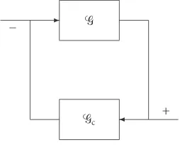
6. Stability of feedback interconnections of discrete-time large-scale nonlinear dynamical systems

In this section, we consider stability of feedback interconnections of discrete-time large-scale nonlinear dynamical systems. Specifically, for the discrete-time large-large-scale dynam-ical systemᏳgiven by (3.1), (3.2), we consider either a dynamic or static discrete-time large-scale feedback systemᏳc. Then, by appropriately combining vector storage