R E S E A R C H
Open Access
Computation of iterative solutions along
with stability analysis to a coupled system of
fractional order differential equations
Sajjad Ali
1, Thabet Abdeljawad
2, Kamal Shah
3*, Fahd Jarad
4and Muhammad Arif
1*Correspondence:
3Department of Mathematics, University of Malakand, Khyber Pakhtunkhwa, Pakistan Full list of author information is available at the end of the article
Abstract
In this research article, we investigate sufficient results for the existence, uniqueness and stability analysis of iterative solutions to a coupled system of the nonlinear fractional differential equations (FDEs) with highier order boundary conditions. The foundation of these sufficient techniques is a combination of the scheme of lower and upper solutions together with the method of monotone iterative technique. With the help of the proposed procedure, the convergence criteria for extremal solutions are smoothly achieved. Furthermore, a major aspect is devoted to the investigation of Ulam–Hyers type stability analysis which is also established. For the verification of our work, we provide some suitable examples along with their graphical represntation and errors estimates.
Keywords: Monotone iterative technique; Fractional differential equations; Extremal solutions; Ulam stability
1 Introduction
FDEs and their systems are the core purpose of most of the researchers because they have many important applications in various fields of advanced technology and science. There are many books and articles which have been written on the topic, see the works of Mainardi and Podlubny. Some applications where FDEs have been used are as follows:
• Modeling materials or systems which are dependent on past history (memory) such as nonlocal elasticity, biological tissues, propagation in complex medium, earth
sediments, polymers, and expansion of the universe. • Strong connection with fractal geometry.
• Can be derived even from probabilistic approaches.
Moreover, classical DEs are just discrete aspects of the whole spectrum of DEs, while FDEs give the total spectrum.
Although some phenomena have been produced in the form of integral order differen-tial equations, in general, every phenomenon cannot be produced accurately in the form of integral order differential equations like the phenomena of electrochemistry, rheology, porous media, geology, electromagnetism, optics, medicine, bioscience, bioengineering, probability, and statistics. In this concern, most of the researchers prefer nonlinear FDEs, which are powerful tools, instead of the integral order differential equations for
ical modeling of the aforesaid phenomena. Therefore, plenty of the research items have been written on nonlinear FDEs, see [1–8] to explore more of their features for modeling purposes. Numerous properties and useful features of mathematical modeling of FDEs have been established by many authors in almost every field of science and technology such as ecology, control theory, seepage flow in porous media, and nonlinear oscillations due to earthquake (for details, see [9–15]). Furthermore, many researchers have devoted their works to the uniqueness and existence of solutions to FDEs; for reading, see [16–20]. As far as we know, the aforesaid area of fractional calculus has been greatly developed. The field of a coupled system of fractional differential equations is the main research field of most of the authors. It is the cascading form of single fractional differential equation. The handling of a coupled system of FDEs is a difficult task as compared with single fractional differential equation. In concern to the establishment of various aspects of the coupled system of FDEs is the need of science and technology because some phenomena describe more than one required task (solution) to be found. These phenomena can be expressed as a system of FDEs instead of DE/FDE. In this regard, some authors have devoted their trea-sured work to basic features and properties of the coupled systems of FDEs; for reading, see [21–24].
Existence and uniqueness of differential equations involving fractional derivatives have been considered in many works. For details on these works, we refer the readers to [25–
31] and the works cited therein. Recently, the existence and uniqueness of lower and upper solutions of FDEs have attracted the focus of most of researchers. Although some authors have well studied lower and upper solutions of integral order partial and ordinary dif-ferential equations using iterative techniques (see [32–42]), the iterative techniques have been rarely studied for the lower and upper solutions of FDEs as well as coupled systems of FDEs. It is a useful tool for the existence of approximation to the solutions of many applied problems of integral and differential equations of arbitrary order. The aforemen-tioned scheme has been studied by some authors for FDEs. Quite recently, Ali [43] has considered this scheme (technique) for the following fractional differential equations:
⎧ ⎨ ⎩
Dαθ(ξ) +f(ξ,θ(ξ)) = 0, ξ∈(0, 1), 1 <α< 2,
θ(0) = 0, θ(1) =ξ θ(),
whereξ,∈(0, 1).
As far as we know, the aforementioned scheme for the coupled system of FDEs is in its initial stage.
The aim of our manuscript is to extend the scheme of Ali [43] to coupled systems of FDEs. We consider the following class of nonlinear fractional coupled system of higher order boundary conditions:
⎧ ⎪ ⎪ ⎪ ⎪ ⎪ ⎨ ⎪ ⎪ ⎪ ⎪ ⎪ ⎩
Dpθ(ξ) +Φξ,ϑ(ξ)= 0, ξ∈[0, 1],
Dqϑ(ξ) +Ψξ,θ(ξ)= 0, ξ∈[0, 1],
θ(1) =θ(0) =θ(0) =· · ·=θ(n–2)(0) =θ(n–1)(0) = 0,
ϑ(1) =ϑ(0) =ϑ(0) =· · ·=ϑ(n–2)(0) =ϑ(n–1)(0) = 0,
(1)
wheren= 2, 3, 4, . . . ,n– 1 <q,p≤n,θ,y∈C[0, 1].
Dis considered in the sense of Caputo derivative assuming thatΦ,Ψ:I×R→R. This manuscript has the following main contributions:
• To extend and develop the iterative scheme while combining the method of lower and upper solutions for the nonlinear fractional coupled system of higher order boundary conditions.
• Existence of lower and upper solutions of the nonlinear fractional coupled system of higher order boundary conditions.
• The investigation of Ulam–Hyers stability for the coupled system of nonlinear FDEs of higher order boundary conditions.
• Approximations of extremal solutions of the nonlinear fractional coupled system of higher order boundary conditions.
• Provision of maximum errors estimate of extremal solutions of the nonlinear fractional coupled system of higher order boundary conditions.
• The presentation of lower and upper solutions of the nonlinear fractional coupled system of higher order boundary conditions via plots using Matlab software.
Three illustrative examples are provided to demonstrate the obtained results. Further we remark that Caputo type fractional order derivative is considered throughout this paper.
2 Background materials
In the present section of our work, we mention supportive basic definitions with useful lemmas from fractional calculus as well as measure theory and functional analysis; for reading, see [2–5,19,20,37].
Definition 2.1 Letθ(ξ)∈L([0, 1],R) be a function. Then the Riemann–Liouville integral of fractional orderδ∈R+of functionθ(ξ) is given by
Iδθ(ξ) = 1 Γ(δ)
ξ
0
(ξ–σ)δ–1θ(σ)dσ,
provided that the integral is pointwise defined on the right-hand side.
Definition 2.2([3]) The Caputo derivative of fractional orderpof functionθ(ξ) is defined by
Dpθ(ξ) = 1
Γ(n–p) ξ
0
provided that the integral on the right-hand side is pointwise defined on (0,∞), where
n= [p] + 1 and [p] denotes the integer part of the real numberp.
Definition 2.3 As in [21,43], “LetU=C[0, 1] be the Banach space endowed withθ=
maxξ∈[0,1]|θ(ξ)|which satisfies the partial ordering, and letW= [θ1,θ2] withθ1≤θ2be
a set such thatW ⊂U, then the operatorT:W→U is known as increasing function if for eachθ1,θ2∈W andθ1≤θ2givesTθ1≤Tθ2. The operatorTis known as decreasing
function if for eachθ1,θ2∈WgivesTθ1≥Tθ2.”
Definition 2.4 As in [21, 43], “Let I be an identity operator. If (I–T)θ1≤0, then the
functionθ1∈W is known as a minimal solution of (I–T)θ = 0 and if (I–T)θ2≥0, then
the functionθ2∈Wis known as a maximal solution of (I–T)θ= 0.”
Lemma 2.5([20]) For the Banach spaceUwhich partially satisfies order with W⊂Uand
θn,θn∗∈W such thatθn≤θn∗,n∈Z+.Ifθn→θ andθn∗→θ∗,thenθ≤θ∗.
Lemma 2.6([3,49]) Let p> 0,then the FDE Dpθ(ξ) = 0
has the solution in the form of
θ(ξ) =
[p]
i=0
θ(i)(0)
i! t
i.
Lemma 2.7([3,49]) Let p> 0,then
IpDpθ(ξ)=θ(ξ) –
[p]
i=0
θ(i)(0)
i! t
i.
3 Iterative solutions
This section is committed to the existence theory, approximation and error estimates to the extremal solution of system (1). In the first attempt we transfer system (1) to the equiv-alent system of integral equations. It is to be noted that the integral representation of the coupled system is very useful for onward computations. Green’s function in the integral representation is also necessary to be computed for iterative solution. The next step af-ter the integral representation is establishing sufficient conditions for the existence of ex-tremal solutions to system (1). We also provide iterative approximation to extremal so-lution of the system by a monotone iterative scheme coupled with the lower and upper solutions method. Further, by the convergent property of monotonic sequence, we con-sequently compute the error estimates for the iterative solution to extremal solutions of system (1). For the aforesaid concerns and computations, the following assumptions are considered:
(C1) The real-valued functionsΦ,Ψ : [0, 1]×R→Rsatisfy the Carathéodory lemma
(for reading, see the preliminary section of [20]).
(C2) The functionsΦ(ξ,θ)and Ψ(ξ,ϑ)are increasing inθ and ϑ for everyξ ∈[0, 1]
(C3) The existence of the constants A,B> 0such that0≤Φ(ξ,θ1(ξ)) –Φ(ξ,θ2(ξ)≤ A(θ1–θ2)and0≤Ψ(ξ,ϑ1(ξ)) –Ψ(ξ,ϑ2(ξ)≤B(ϑ1–ϑ2).
Lemma 3.1 In view of C1with h∈C([0, 1],R),then the fractional differential equation
Dpθ(ξ) +h(ξ) = 0, ξ∈[0, 1], (n– 1) <p≤n,
θ(1) =θ(0) =θ(0) =· · ·=θ(n–2)(0) =θ(n–1)(0) = 0
(2)
has the solution defined by
θ(ξ) = 1
0
G1(ξ,σ)h(σ)dσ, (3)
whereG1(ξ,σ)is given by
G1(ξ,σ) =
1 Γ(p)
⎧ ⎨ ⎩
(1 –σ)p–1– (ξ–σ)p–1, 0≤σ≤ξ≤1,
(1 –σ)p–1, 0≤ξ≤σ≤1.
(4)
G1(ξ,σ)is known as Green’s function.
Proof In view of Lemma2.7and derivative considered in the sense of Caputo derivative, the linear BVP (2) yields that
θ(ξ) =C1+C2ξ+· · ·+Cnξn–1–Iph(ξ). (5)
We face singularity by using the conditionsθ(0) =θ(0) =· · ·=θ(n–2)(0) =θ(n–1)(0) = 0. Therefore to avoid singularity, here we haveC2=C3=C4=· · ·=Cn= 0. Further, asθ(1) =
0, then we haveC1=Iph(1). Therefore, we deduce from (5) that
θ(ξ) = 1
0
(1 –σ)p–1
Γ(p) h(σ)dσ– ξ
0
(ξ–σ)p–1
Γ(p) h(σ)dσ. (6)
Hence, we obtain the result from (6) that is
θ(ξ) = 1
0
G1(ξ,σ)h(σ)dσ.
This is the end of the proof.
Lemma 3.2 Let W =C[0, 1]be the Banach space withθ=maxξ∈[0,1]|θ(ξ)|.Then the
coupled system(1)has the integral representation
⎧ ⎨ ⎩
θ(ξ) =01G1(ξ,σ)Φ(σ,ϑ(σ))dσ, ξ∈[0, 1],
ϑ(ξ) =01G2(ξ,σ)Ψ(σ,θ(σ))dσ, ξ∈[0, 1],
(7)
whereG1(ξ,σ)is given in(4)and
G2(ξ,σ) =
⎧ ⎨ ⎩
(1–σ)q–1–(ξ–σ)q–1
Γ(q) , 0≤σ≤ξ≤1,
(1–σ)q–1
Clearly,G1(ξ,σ)≥0,G2(ξ,σ)≥0 for allξ,σ∈[0, 1].
Lemma 3.3 The functionsG1,G2satisfy the following property:
1
Hence, the proof is completed.
We write the coupled system (7) of integral equations as
θ(ξ) =
Thanks to equation (8) and equation (9), we obtain the equation
It is to be noted that equations (8) and (10) have the same solutions that are fixed points
thusTis an increasing operator.
(C4) Assume that the lower and upper solutions of (10) areα and β ∈W. Then the
inequalityα≤βon[0, 1]holds.
Lemma 3.4 Consider all the assumptions(C1)to(C4).Then the solutions of linear
prob-lems are an iterative convergent sequence which converges to solution of the integral equa-tion(8).
Therefore, the operator T is continuous. Further, it is obvious that T is also equi-continuous and uniformly bounded. Arzelá–Ascoli theorem which states that “IfMis a family (finite or infinite) of an equi-continuous, uniformly bounded real-valued functions θ on an interval [0, 1], thenMcontains a uniformly convergent sequence of functionsθn,
converging to a functionθinWasn→ ∞, whereWdenotes the space of all continuous bounded functions on [0, 1]. Thus any sequence inMcontains a uniformly bounded con-vergent subsequence on [0, 1] and consequentlyMhas a compact closure inW.” Hence, in view of the Arzelá–Ascoli theorem,Tis also a compact operator. Let the lower solution of integral equation (10) beθ0=α. Then, in view of condition (C4), we obtain
AsTis an increasing operator, then we obtain
θ0≤Tθ0≤Tβ≤β, that is,θ0≤θ1≤βon the interval [0, 1],
whereθ1=Tθ0is an iterative solution of integral equation (10). By applyingT, we obtain Tθ0≤Tθ1≤Tβ≤β, that is,θ1≤θ2≤βon [0, 1],
whereθ2=Tθ1. Consequently, we obtain a bounded monotone sequence{θn}which is
θ0≤θ1≤θ2≤ · · · ≤θn–1≤θn≤β on [0, 1], (13)
whereθn=Tθn–1 is solution of equation (10). Thus, in view of the bounded monotone
sequence{θn}, there existsθ ∈Wso thatθn→θ asn→ ∞. Thereforeθ =Tθ, which is
the solution of integral equation (8) defined by
θ(ξ) = 1
0
G1(ξ,σ)Φ
σ,
1
0
G2(σ,)Ψ
,θ()d
dσ, ξ∈[0, 1].
Hence, in view of (13) and (12), we get
θ2–θ1=Tθ1–Tθ0 ≤ ∇e1,
θ3–θ2=Tθ2–Tθ1 ≤ ∇2e1,
θ4–θ3=Tθ3–Tθ2 ≤ ∇3e1,
.. .
θn+1–θn=Tθn–Tθn–1 ≤ ∇ne1.
Consequently, for positive integersmandn, we have
θm+n–θn ≤ θn+m–θn+m–1+θn+m–1–θn+m–2+· · ·+θn+1–θn
≤ ∇n1 –∇m
1 –∇ e1. (14)
It is obvious that∇< 1, which implies thatθm+n–θn →0 whenn→ ∞. Thusθnis a
Cauchy sequence inW. Letθ∗(ξ) =limn→∞θn(ξ), thusTθ∗=θ∗. Therefore, ifm→ ∞in
(14), then error estimate for the lower solution is
en=θ∗–θn≤
∇n
1 –∇e1, wheree1=θ1–θ0.
Remark Let us chooseθ0=β, we have a sequence{θn}so that
θ0≥θ1≥θ2≥ · · · ≥θn–1≥θn≥α on [0, 1],
wheree∗1=θ0∗–θ1∗. Further, we use Lemma3.4, the iterative sequences for lower and upper solutions of system (1) are:
θn(ξ) =
of BVPs(1)has unique minimal and maximal solutions respectively.
Proof We prove that (θ∗,ϑ∗) and (θ¯∗,ϑ¯∗) are the minimal and maximal solutions of (7). Let for anyu(ξ)∈WwithTu=uandθn≤u≤θn∗, due to the increasing behavior ofTand
using Lemma3.4, we haveθ∗(ξ)≤u(ξ)≤ ¯θ∗(ξ) thatθ∗(ξ) andθ∗¯(ξ) are the minimal and maximal fixed points ofTrespectively. Therefore (θ∗,ϑ∗) and (θ¯∗,ϑ¯∗) are the minimal and maximal solution of (7) respectively.
Next, for the concern of uniqueness of minimal and maximal solutions of system (7), let α,β∈Wbe the lower and upper solutions ofTθ=θ respectively. Thenα≤Tα,β≥Tβ, minimal and maximal solutions of the coupled system (7) are unique.
4 Generalized Ulam–Hyers stability of the solutions of BVPs (1)
This section is devoted to the investigation of more general stability analysis for the sys-tem of fractional differential equations. The stability analysis is an important aspect of fractional calculus for the ordinary and partial differential equations of fractional order. As far as we know, it is in the initial stage for a coupled system. Therefore the aim of this section is to investigate some sufficient conditions for a system of fractional differential equations. In this concern, we study Ulam–Hyers and generalized Ulam–Hyers stability for a coupled system of BVPs (1) of the nonlinear FDEs. For this concern, we require the following auxiliary definitions.
ε2> 0 and for every solution (θ,ϑ)∈C([0, 1], R)×C([0, 1], R) of the inequality
Dpθ(ξ) –Φξ,ϑ(ξ)≤ε
1, ξ∈[0, 1],
Dqϑ(ξ) –Ψξ,θ(ξ)≤ε
2, ξ∈[0, 1],
(15)
there exists a unique solution (θ˜,ϑ)˜ ∈C([0, 1], R)×C([0, 1], R) of the proposed BVPs (1) with
(θ,ϑ) – (θ˜,ϑ)˜ ≤ ˆCΦ,Ψε, ξ∈[0, 1].
Definition 4.2 The proposed BVPs (1) is called to be generalized Ulam–Hyers stable if we can find ΘΦ,Ψ : (0,∞)→R+ with ΘΦ,Ψ(0) = 0, with the property that, for every
ε=max{ε1,ε2}> 0 with ε1> 0 andε2 > 0 and for every solution (θ,ϑ)∈C([0, 1], R)×
C([0, 1], R) of the inequality
Dpθ(ξ) –Φξ,ϑ(ξ)≤ε
1, ξ∈[0, 1],
Dqϑ(ξ) –Ψξ,θ(ξ)≤ε
2, ξ∈[0, 1],
there exists a unique solution (θ˜,ϑ)˜ ∈C([0, 1], R)×C([0, 1], R) of the proposed BVPs (1) with
(θ,ϑ) – (θ˜,ϑ)˜ ≤ ˆCΦ,ΨΘΦ,Ψ(ξ), ξ∈[0, 1].
Remark4.3 The (θ,ϑ)∈C([0, 1],R) is said to be the solution of BVPs (1) and satisfy the inequality given in (15) if and only if we can find a functionα,β∈C([0, 1],R) depending only on (θ,ϑ) respectively, then
(i) |α(ξ)| ≤ε1,|β(ξ)| ≤ε2, for allξ∈[0, 1];
(ii) Dpθ(ξ) +Φ(ξ,ϑ(ξ)) =α(ξ), for allξ∈[0, 1],Dqϑ(ξ) +Ψ(ξ,θ(ξ)) =β(ξ), for all ξ∈[0, 1].
Thanks to Remark4.3and assumption (C3) forξ∈([0, 1]), the considered solution (θ,ϑ)
of the problem
⎧ ⎪ ⎪ ⎪ ⎪ ⎪ ⎨ ⎪ ⎪ ⎪ ⎪ ⎪ ⎩
Dpθ(ξ) +Φ(ξ,ϑ(ξ)) =α(ξ), ξ∈[0, 1],
Dqϑ(ξ) +Ψ(ξ,θ(ξ)) =β(ξ), ξ∈[0, 1],
given by
Theorem 4.4 Let∇< 1and assumption(C3)hold.Then solutions of the considered
cou-pled system(1)are Ulam–Hyers stable and consequently generalized Ulam–Hyers stable.
Proof Let (θ,ϑ) be any solution of BVPs (1)and satisfy inequality (15), and let (θ¯,ϑ) be the¯ unique solution of the considered BVPs problem, then consider
|θ–θ¯|
Therefore from inequality (19)
In the same manner, it is easy to prove that
ϑ–ϑ¯ ≤ε1CˆΨ, CˆΨ =
1
(1 –∇)Γ(q+ 1)> 0. (21)
Therefore, from inequalities (20) and (21), we have
(θ,ϑ) – (θ¯,ϑ)¯ ≤max{ε1CˆΦ,ε2CˆΨ}=εCˆΦ,Ψ. (22)
Therefore the solutions of a coupled system of BVPs (1) are Ulam–Hyers stable. Further, ifΘΦ,Ψ(ε) =ε, hence (22) can be expressed as
(θ,ϑ) – (θ¯,ϑ)¯ ≤ ˆCΦ,ΨΘΦ,Ψ(ε). (23)
Therefore,ΘΦ,Ψ(0) = 0 in (23) holds. Thus, solutions of the system of BVP (1) are
general-ized Ulam–Hyers stable. Thus we have investigated sufficient condition for Ulam–Hyers stability generalized Ulam–Hyers stability, that is,∇< 1.
5 Examples
In this section, we provide some examples of the coupled system (1). We compute the it-erative approximation for the extremal solution of the corresponding examples. We also provide error estimates for the extremal solutions. Furthermore, the stability analysis un-der the sufficient conditions for the examples of system (1) is also the concern of this section. We also provide the plots of each example of system (1) in the frame figures.
Example5.1 Consider the following coupled system of BVPs of FDEs:
D52θ(ξ) +t 7
2ϑ(ξ)(56,754ϑ2(ξ) + 160)
1 +ϑ2(ξ) = 0, 0≤ξ≤1,
D2710ϑ(ξ) +t 9
2θ(ξ)(θ(ξ) + 1)(23,471e(–θ(ξ))+ 120)
2 +θ(ξ) = 0, 0≤ξ≤1,
(24)
under the boundary condition given by
θ(1) =θ(0) =θ(0) = 0, ϑ(1) =ϑ(0) =ϑ(0) = 0. (25)
As forA=B= 0.0001, we have∇= 7.2147e–10< 1. Whenn= 3 is large enough, iterative
sequences for the approximate minimal and maximal solutionsθnandθ¯n∗respectively are:
θ∗(ξ) =θ3(ξ),
ϑ∗(ξ) = 1
0
G2(ξ,σ)
σ92θ2(σ)(θ2(σ) + 1)(23,471e–θ2(σ)+ 120)
1 +θ2(σ)
dσ,
¯
θ∗(ξ) =θ3∗(ξ),
¯
ϑ∗(ξ) = 1
0
G2(ξ,σ)
σ92θ∗
2(σ)(θ2∗(σ) + 1)(23,471e–θ ∗
2(σ)+ 120)
1 +θ2∗(σ) dσ.
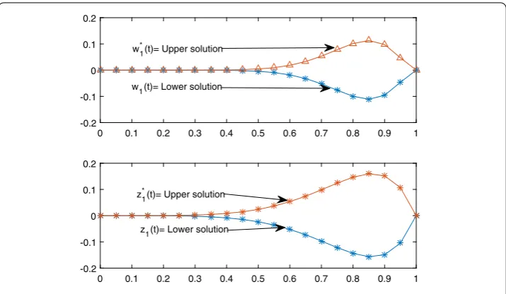
Figure 1A line graph of the solutions of Example5.1
Let (θ0,ϑ0) = (–0.01, –0.01), (θ0∗,ϑ0∗) = (0.01, 0.01) be the minimal and maximal solutions
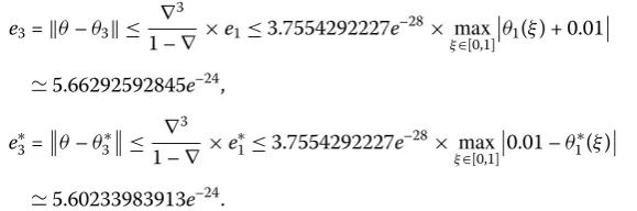
of Example5.1respectively, then we have their corresponding maximum error estimates:
e3=θ–θ3 ≤ ∇ 3
1 –∇ ×e1≤3.7554292227e
–28× max
ξ∈[0,1]
θ1(ξ) + 0.01
5.66292592845e–24,
e∗3=θ–θ3∗≤ ∇
3
1 –∇ ×e ∗
1≤3.7554292227e–28×ξmax∈ [0,1]
0.01 –θ1∗(ξ)
5.60233983913e–24.
The iterative solutions of minimal and maximal of Example5.1are plotted in Figs.1–2
wherein for the simple execution of Matlab code, we have replaced (θ,ϑ) by (w,z) and (θ∗,ϑ∗) by (w∗,z∗). Each plot in the figures has the demonstration of physical behavior of the approximate solutions.
Further, as ∇ < 1, therefore, the Ulam–Hyers stability and generalized Ulam–Hyers stability are obvious. The stability of the iterative solutions can also be observed from Figs.1–2.
Example5.2 To strengthen our results, we provide another example as follows:
D195θ(ξ) +
1 +ϑ2(ξ)ϑ1.1(ξ) +ϑ2.3(ξ)= 0, 0≤ξ≤1,
D7
2ϑ(ξ) +θ(ξ)θ2.3(ξ) +θ1.1(ξ)= 0, 0≤ξ≤1,
(27)
subject to boundary conditions given as
Figure 2A line graph of the solutions of Example5.1, whenp=115 andq=157
As forA=B= 641, we have∇ = 1.1767e–6< 1. Whenn= 3 is large enough, iterative
se-quences for the approximate minimal and maximal solutionsθnandθ¯n∗respectively are:
θ∗(ξ) =θ3(ξ), ϑ∗(ξ) =
1
0 G
2(ξ,σ)
θ2(σ)
θ22.3(σ) +θ21.1(σ)dσ,
¯
θ∗(ξ) =θ3∗(ξ), ϑ¯∗(ξ) = 1
0
G2(ξ,σ)
θ2∗(σ)θ2∗(σ)2.3+θ2∗(σ)1.1dσ.
(29)
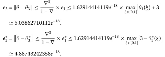
Let (θ0,ϑ0) = (–3, –3), (θ0∗,ϑ0∗) = (3, 3) be the maximal and minimal solutions of
Exam-ple5.2respectively, then the error estimates are:
e3=θ–θ3 ≤ ∇ 3
1 –∇ ×e1≤1.62914414119e
–18× max
ξ∈[0,1]
θ1(ξ) + 3
5.03862710112e–18,
e∗3=θ–θ3∗≤ ∇
3
1 –∇ ×e ∗
1≤1.62914414119e–18× max ξ∈[0,1]
3 –θ1∗(ξ)
4.88743242358e–18.
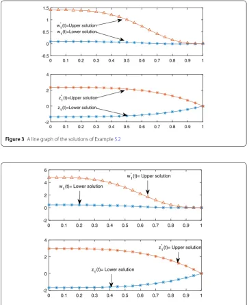
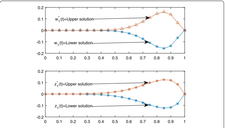
The iterative solutions of minimal and maximal of Example5.2are plotted in Figs.3–4, wherein for the simple execution of Matlab code, we have replaced (θ,ϑ) by (w,z) and (θ∗,ϑ∗) by (w∗,z∗). Each plot in the figures has the demonstration of physical behavior of the approximate solutions.
Figure 3A line graph of the solutions of Example5.2
Figure 4A line graph of the solutions of Example5.2, whenp=17 5 andq=
10 3
Example5.3 Consider the following coupled system of BVPs of FDEs:
D215θ(ξ) +t 15
4ϑ(ξ)(ϑ2(ξ) + 160)
(1 +ϑ2(ξ))2 = 0, 0≤ξ≤1,
D92ϑ(ξ) +t 19
4 θ(ξ)(θ(ξ) + 1)(θ(ξ) + 9)(e–2θ(ξ)+ 120)
(2 +θ(ξ))2 = 0, 0≤ξ≤1,
(30)
with the given boundary condition
θ(1) =θ(0) =θ(0) =θ(0) =θ(0) = 0,
ϑ(1) =ϑ(0) =ϑ(0) =ϑ(0) =ϑ(0) = 0.
Obviously,A=B=641, from which it is easy to see that∇= 1.4317e–7< 1. For takingn= 3
is large enough, we have the iterative sequences for approximate minimal and maximal solutionsθnandθ¯n∗as given by
θ∗(ξ) =θ3(ξ),
ϑ∗(ξ) = 1
0
G2(ξ,σ)
σ194θ2(σ)(θ2(σ) + 1)(θ2(σ) + 9)(e–2θ2(σ)+ 120)
(2 +θ2(σ))2
dσ,
¯
θ∗(ξ) =θ3∗(ξ),
¯
ϑ∗(ξ) = 1
0
G2(ξ,σ)
t194θ∗
2(σ)(θ2∗(σ) + 1)(θ2∗(σ) + 9)(e–2θ ∗
2(σ)+ 120)
(2 +θ2∗(σ))2 dσ,
(32)
respectively. Let (θ0,ϑ0) = (–0.1, –0.1), (θ0∗,ϑ0∗) = (0.1, 0.1) be maximal and minimal
solu-tions respectively of Example5.3, then
e3=θ–θ3 ≤
∇3
1 –∇ ×e1≤2.93476154975e
–21× max
ξ∈[0,1]
θ1(ξ) + 0.1
2.93476154975e–22,
e∗3=θ–θ3∗≤ ∇
3
1 –∇ ×e ∗
1≤2.93476154975e–21× max ξ∈[0,1]
0.1 –θ1∗(ξ)
2.93476154975e–22.
Physical behavior of the approximate maximal and minimal solutions has also been demonstrated by providing Figs.5–6, wherein, for the simple execution of Matlab code, we have replaced (θ,ϑ) by (w,z) and (θ∗,ϑ∗) by (w∗,z∗).
It is easy to obtain the conditions of various types of Ulam–Hyers stabilities for the so-lutions. The stability of iterative solutions is also obvious from Figs.5–6.
Figure 6A line graph of the solutions of Example5.3, whenp=235 andq=133
Figures discussion: We have plotted the iterative solutions of three considered exam-ples of system (1). These plots are provided in Figs.1–6. For the sketch of plots, we have used the subplot command in the Matlab software. Each plot of numerical results shows a meaningful behavior of the extremal solutions of the coupled system of fractional differ-ential equations. The different visualizations of each upper and lower solutions are very clear.
6 Conclusion
We have developed sufficient conditions for the existence of extremal solutions to a cou-pled system of FDEs with highier order boundary conditions. We have successfully pro-vided these sufficient conditions on the basis of combining the method of upper and lower solutions together with the method of monotone iterative technique. We have constructed two monotonic sequences corresponding to upper and lower solutions such that a mono-tonically increasing sequence converged to the maximal solutions and the monomono-tonically decreasing sequence converged to the minimal solutions of the system under considera-tion. Finally, an error estimate has been established, which provided the efficiency of the method.
Acknowledgements
Further we are thankful to the anonymous referee for useful suggestions.
Funding
The second author would like to thank Prince Sultan University for funding this work through research group Nonlinear Analysis Methods in Applied Mathematics (NAMAM), group number RG-DES-2017-01-17.
Abbreviations
FDEs; BVPs
Availability of data and materials
Not applicable.
Competing interests
Authors’ contributions
All authors have done equal contribution in this article. All authors read and approved the final manuscript.
Author details
1Department of Mathematics, Abdul Wali Khan University Mardan, Khyber Pakhtunkhwa, Pakistan.2Department of Mathematics and General Sciences, Prince Sultan University, Riyadh, Saudi Arabia. 3Department of Mathematics, University of Malakand, Khyber Pakhtunkhwa, Pakistan. 4Department of Mathematics, Çankaya University, Ankara, Turkey.
Publisher’s Note
Springer Nature remains neutral with regard to jurisdictional claims in published maps and institutional affiliations.
Received: 6 February 2019 Accepted: 21 May 2019 References
1. Kilbas, A.A., Marichev, O.I., Samko, S.G.: Fractional Integrals and Derivatives (Theory and Applications). Gordon and Breach, Switzerland (1993)
2. Miller, K.S., Ross, B.: An Introduction to the Fractional Calculus and Fractional Differential Equations. Wiley, New York (1993)
3. Podlubny, I.: Fractional Differential Equations, Mathematics in Science and Engineering. Academic Press, New York (1999)
4. Hilfer, R.: Applications of Fractional Calculus in Physics. World Scientific, Singapore (2000)
5. Kilbas, A.A., Srivastava, H.M., Trujillo, J.J.: Theory and Applications of Fractional Differential Equations. Elsevier, Amsterdam (2006)
6. Benchohra, M., Graef, J.R., Hamani, S.: Existence results for boundary value problems with nonlinear fractional differential equations. Appl. Anal.87, 851–863 (2008)
7. Agarwal, R.P., Belmekki, M., Benchohra, M.: A survey on semilinear differential equations and inclusions involving Riemann–Liouville fractional derivative. Adv. Differ. Equ.2009, Article ID 981728 (2009)
8. Agarwal, R.P., Benchohra, M., Hamani, S.: A survey on existence results for boundary value problems of nonlinear fractional differential equations and inclusions. Acta Appl. Math.109, 973–1033 (2012)
9. Abbas, S., Benchohra, M.: Topics in Fractional Differential Equations. Springer, Berlin (2012) 12 pages 10. Benchohra, M., Graef, J.R., Hamani, S.: Existence results for boundary value problems with non-linear fractional
differential equations. Appl. Anal.87(7), 851–863 (2008)
11. Isaia, F.: On a nonlinear integral equation without compactness. Acta Math. Univ. Comen.iv, 233–240 (2006) 12. Kilbas, A.A., Marichev, O.I., Samko, S.G.: Fractional Integrals and Derivatives (Theory and Applications). Gordon and
Breach, Switzerland (1993)
13. Miller, K.S., Ross, B.: An Introduction to the Fractional Calculus and Fractional Differential Equations. Wiley, New York (1993)
14. Timoshenko, S.P.: Theory of Elastic Stability. McGraw-Hill, New York (1961) 15. Soedel, W.: Vibrations of Shells and Plates. Dekker, New York (1993)
16. Yang, W.: Positive solution to nonzero boundary values problem for a coupled system of nonlinear fractional differential equations. Comput. Math. Appl.63, 288–297 (2012)
17. Wang, J., Xiang, H., Liu, Z.: Positive solution to nonzero boundary values problem for a coupled system of nonlinear fractional differential equations. Int. J. Differ. Equ.2010, Article ID 186928 (2010)
18. Su, X.: Boundary value problem for a coupled system of nonlinear fractional differential equations. Appl. Math. Lett.
22, 64–69 (2009)
19. Wang, G., Agarwal, R.P., Cabada, A.: Existence results and the monotone iterative technique for systems of nonlinear fractional differential equations. Appl. Math. Lett.25(6), 1019–1024 (2012)
20. Zeidler, E.: Nonlinear Functional Analysis and Its Applications, Part II/B: Nonlinear Monotone Operators. Springer, New York (1989)
21. Shah, K., Khan, R.A.: Iterative solutions to a coupled system of nonlinear fractional differential equations. J. Fract. Calc. Appl.7(2), 40–50 (2016)
22. Shah, K., Khalil, H., Khan, R.A.: Upper and lower solutions to a coupled system of nonlinear fractional differential equations. Prog. Fract. Differ. Appl.1(1), 1–10 (2016)
23. Ahmad, B., Nieto, J.J.: Existence results for a coupled system of nonlinear fractional differential equations with three-point boundary conditions. Comput. Math. Appl.58, 1838–1843 (2009)
24. Gafiychuk, V., Datsko, B., Meleshko, V., Blackmore, D.: Analysis of the solutions of coupled nonlinear fractional reaction-diffusion equations. Chaos Solitons Fractals41, 1095–1104 (2009)
25. Arshad, A., Shah, K., Jarad, F., Gupta, V., Abdeljawad, T.: Existence and stability analysis to a coupled system of implicit type impulsive boundary value problems of fractional-order differential equations. Adv. Differ. Equ.2019, 101 (2019) 26. Jarad, F., Abdeljawad, T., Hammouch, Z.: On a class of ordinary differential equations in the frame of
Atangana–Baleanu fractional derivative. Chaos Solitons Fractals117, 16–20 (2019)
27. Gambo, Y.Y., Ameen, R., Jarad, F., Abdeljawad, T.: Existence and uniqueness of solutions to fractional differential equations in the frame of generalized Caputo fractional derivatives. Adv. Differ. Equ.2018, 134 (2018)
28. Ameen, R., Jarad, F., Abdeljawad, T.: Ulam stability for delay fractional differential equations with a generalized Caputo derivative. Filomat32(15), 5265–5274 (2018)
29. Adjabi, Y., Jarad, F., Baleanu, D., Abdeljawad, T.: On Cauchy problems with Caputo Hadamard fractional derivatives. J. Comput. Anal. Appl.21(4), 661–681 (2016)
30. Abdeljawad, T., Jarad, F., Baleanu, D.: On the existence and the uniqueness theorem for fractional differential equations with bounded delay within Caputo derivatives. Sci. China Ser. A, Math.51(10), 1775–1786 (2008) 31. Abdeljawad, T., Baleanu, D., Jarad, F.: Existence and uniqueness theorem for a class of delay differential equations with
32. Ladde, G.S., Lakshmikantham, V., Vatsala, A.S.: Monotone Iterative Technique for Nonlinear Differential Equations. Pitman Publishing Inc., Boston (1985)
33. Bai, C., Fang, J.: The existence of a positive solution for a singular coupled system of nonlinear fractional differential equations. Comput. Math. Appl.150, 611–621 (2004)
34. Zhang, S.: Monotone iterative method for initial value problem involving Riemann–Liouville fractional derivatives. Nonlinear Anal., Theory Methods Appl.71(5), 2087–2093 (2009)
35. Mcrae, F.A.: Monotone iterative technique and existence results for fractional differential equations. Nonlinear Anal., Theory Methods Appl.71(12), 6093–6096 (2009)
36. Al-Refai, M., Ali Hajji, M.: Monotone iterative sequences for nonlinear boundary value problems of fractional order. Nonlinear Anal., Theory Methods Appl.74(11), 3531–3539 (2011)
37. Xu, N., Liu, W.: Iterative solutions for a coupled system of fractional differential-integral equations with two-point boundary conditions. Appl. Math. Comput.244, 903–911 (2014)
38. Liu, X., Jia, M.: Multiple solutions for fractional differential equations with nonlinear boundary conditions. Comput. Math. Appl.59, 2880–2886 (2010)
39. He, Z., He, X.: Monotone iterative technique for impulsive integro-differential equations with periodic boundary conditions. Comput. Math. Appl.48, 73–84 (2004)
40. De Coster, C., Habets, P.: Two-Point Boundary Value Problems: Lower and Upper Solutions. Elsevier, Amsterdam (2006) 41. Li, F., Jia, M., Liu, X., Li, C., Li, G.: Existence and uniqueness of solutions of second-order three-point boundary value
problems with upper and lower solutions in the reverse order. Nonlinear Anal., Theory Methods Appl.68, 2381–2388 (2008)
42. Hirstova, S., Tunç, C.: Stability of nonlinear Volterra integro-differential equations with Caputo fractional derivative and bounded delays. Electron. J. Differ. Equ.30, 1 (2019)
43. Ali, S., Shah, K., Jarad, F.: On stable iterative solutions for a class of boundary value problem of nonlinear fractional order differential equations. Math. Methods Appl. Sci.42(3), 969–981 (2019)
44. Rus, I.A.: Ulam stabilities of ordinary differential equations in a Banach space. Carpath. J. Math.26, 103–107 (2010) 45. Rassias, T.M.: On the stability of the linear mapping in Banach spaces. Proc. Am. Math. Soc.72, 297–300 (1978) 46. Rassias, T.M.: On the stability of functional equations and a problem of Ulam. Acta Appl. Math.26, 23–130 (2000) 47. Hirstova, S., Tunç, C.: Stability of nonlinear Volterra integro-differential equations with Caputo fractional derivative
and bounded delays. Electron. J. Differ. Equ.30, 1 (2019)
48. Wang, J., Feˇckan, M., Zhou, Y.: Fractional order differential switched systems with coupled nonlocal initial and impulsive conditions. Bull. Sci. Math.141, 727–746 (2017)