Envelope syntheses of cylindrical vector-waves in 2-D random elastic media
based on the Markov approximation
Haruo Sato1and Michael Korn2
1Department of Geophysics, Graduate School of Science, Tohoku University, Aramaki-Aza-Aoba 6-3, Aoba-ku,
Sendai-shi, Miyagi-ken, 980-8578, Japan
2Institute of Geophysics and Geology, University of Leipzig, Talstrasse 35, 04103 Leipzig, Germany (Received May 11, 2006; Revised November 2, 2006; Accepted December 4, 2006; Online published May 7, 2007)
Seismograms of microearthquakes are complex; however, their envelopes broaden as the travel distance increases.P-waves are recorded in transverse components,S-waves are recorded in the longitudinal component, and waves are observed at sites even in the nodal direction of the source radiation. These phenomena, which are typically found in short-period seismograms, can be interpreted to be the result of scattering due to lithospheric inhomogeneity. We report here our study of a simple statistical model in which the propagation of waves radiated from a point source in two-dimensional (2-D) random elastic media is characterized by a Gaussian autocorrelation function. For the case that the wavelength is shorter than the correlation distance, two methods based on the Markov approximation are introduced for the direct synthesis of vector wave envelopes. One is to analytically solve the stochastic equation for the two-frequency mutual coherence function; the validity of the solution is confirmed by using finite difference simulations. The second is to numerically solve the stochastic equation for the mutual coherence function. The two methods are equivalent, but the latter is applicable to nonisotropic source radiation. For the case of a point shear dislocation source, a peak delay from the onset and a smoothly decaying tail are found to be common to synthesized envelopes in all azimuths. Scattered waves are excited even at receivers in the nodal direction, and amplitudes become independent of the radiation pattern as lapse time increases.
Key words:Scattering, random media, envelope, simulation.
1.
Introduction
Seismic observations of local microearthquakes have re-vealed that high-frequency seismograms are strongly de-formed by the propagation process through the randomly inhomogeneous structure of the lithosphere. In addition to the excitation of coda waves (Aki and Chouet, 1975), P -waves are seen in transverse components,S-waves are also seen in the longitudinal component (Matsumura and Sato, 1981), and waves are observed at sites even in the nodal direction of source radiation. Peak delay and the broaden-ing of the envelope with increasbroaden-ing travel distance are also direct evidence of wave scattering due to medium inhomo-geneity (Sato, 1989).
There have been developments in the modeling of wave envelopes in random media and analysis of observed seis-mogram envelopes (see Sato and Fehler, 1998). Complex waveforms have been deterministically and numerically simulated in inhomogeneous media (Frankel and Clayton, 1986; Yomogida and Benites, 1995). On the other hand, the radiative transfer theory with the statistical characterization of medium inhomogeneity has been often used as the ba-sic framework of the envelope synthesis of high-frequency seismograms. Most of these studies treat energy
propaga-Copyright cThe Society of Geomagnetism and Earth, Planetary and Space Sci-ences (SGEPSS); The Seismological Society of Japan; The Volcanological Society of Japan; The Geodetic Society of Japan; The Japanese Society for Planetary Sci-ences; TERRAPUB.
tion focusing on the coda portion of seismogram envelopes with the assumption of isotropic scattering (Sato, 1977; Zeng et al., 1993). Sato et al. (1997) provided an exact solution to the radiative transfer equation for isotropic scat-tering and a point shear dislocation source. This solution has been used in the inversion of strong motion records for the high-frequency radiation from an earthquake fault (see Nakaharaet al., 1998); however, isotropic scattering assumption is not suitable for the envelope near the direct arrival where strong forward scattering dominates. There have been attempts to synthesize polarized vector wave en-velopes, including the studies of Bal and Moscoso (2000), who analyzed the depolarization ofS-waves after multiple scattering, and of Margerinet al.(2000), who synthesized envelopes by using scattering amplitudes of spherical inclu-sions distributed in uniform media and Stokes vectors. The radiative transfer theory is heuristic, but some studies have introduced scattering coefficients predicted from velocity inhomogeneity spectrum by using the Born approximation. Sato (1984) simulated three-component envelopes in ran-dom elastic media for a point shear dislocation source in the framework of single scattering approximation. Gusev and Abubakirov (1996) studied how the degree of nonisotropic scattering affects envelope shape. Recently, Przybillaet al. (2006) showed an excellent coincidence of envelopes syn-thesized by using the Monte Carlo method for the radiative transfer theory and those calculated from finite difference simulations in two-dimension (2-D) random elastic media.
These researchers used scattering amplitudes derived from the Born approximation with the wandering effect of travel time.
When the wavelength is smaller than the characteristic scale of medium inhomogeneity, conversion scattering is weak and scattering occurs around the forward direction, where the parabolic approximation is suitable for the syn-thesis of waves near the direct arrival. In this case, en-velopes in random media can be well synthesized by the Markov approximation for the two-frequency mutual coher-ence function (TFMCF), which is a stochastic extension of the phase screen method (Ishimaru, 1978). Sato (1989) ap-plied its solution for the interpretation of envelope broaden-ing of observedS-wave seismograms in Kanto, Japan. Saito et al. (2002) theoretically solved the envelope broadening of spherically outgoing waves in von K´arm´an-type 3-D ran-dom media that have a realistic power-law spectrum at large wavenumbers. Fehleret al.(2000) confirmed the validity of the Markov approximation for scalar waves from a compari-son with finite difference simulations in 2-D random media. Wegleret al.(2006) numerically examined the applicable range of the Markov approximation, and the radiative trans-fer solution with Born scattering amplitudes and that with isotropic scattering for scalar waves taking the finite differ-ence simulation envelope as a referdiffer-ence in 2-D random me-dia. Compared with the radiative transfer theory with Born scattering amplitudes, the Markov approximation method can not explain conversion scattering; however, if we fo-cus on wave envelopes near the direct arrival, this approx-imation has the advantage that the envelope characteristics can be well described by a small number of statistical pa-rameters. Extension of the Markov approximation to vector wave envelopes has been carried out recently by Korn and Sato (2005) and Sato (2006, 2007), who established a rig-orous derivation of vector wave envelopes in random elastic media characterized by a Gaussian autocorrelation function (ACF) that uses the TFMCF of potential field. The valid-ity of the Markov approximation for vector waves was con-firmed from a comparison with finite difference simulations only for plane wave envelopes in the 2-D case (Korn and Sato, 2005).
There is yet another envelope synthesis, called the stochastic ray path method (Williamson, 1972, 1975), which is based on the joint use of the Markov approxi-mation for the mutual coherence function (MCF) and ray travel times. The Monte Carlo method commonly used for the envelope simulation based on the radiative transfer the-ory treats travel distance and scattering angle as stochastic processes (Hoshiba, 1994; Yoshimoto, 2000). In contrast, the stochastic ray path method treats ray bending angle as a stochastic process and interprets the distribution of the ac-cumulated travel times arriving at a given distance as the time trace of wave intensity. This method has the advantage that it is easily applicable to nonisotropic source radiation. In addition, it needs a relatively small number of shots for a stable estimation of envelopes compared with the conven-tional Monte Carlo method based on the radiative transfer theory.
In this paper, we report the results of a basic study of vec-tor seismograms of micro-earthquakes in the lithospheric
inhomogeneity. To this end, we mathematically simulate vector-wave envelopes for a point source radiation in 2-D random elastic media characterized by a Gaussian ACF. Using the Markov approximation for the TFMCF of poten-tial, we solve vector wave envelopes for isotropic radiation from a point source. The synthesized envelopes are then compared with the ensemble-averaged envelopes of finite difference simulations. Next, using the Markov approxi-mation for the MCF of potential, we derive the stochastic master equation appropriate for cylindrical waves. Using the stochastic ray path method—that is, numerically solv-ing this equation and ussolv-ing ray travel times—we synthe-size vector wave envelopes. The equality of two simula-tion methods of the Markov approximasimula-tion is numerically confirmed for the case of isotropic radiation from a point source. Finally, applying the stochastic ray path method to the radiation from a point shear dislocation source, we synthesize vector wave envelopes at receivers in different azimuths.
2.
Markov Approximation for the Two-Frequency
Mutual Coherence Function
2.1 Two-frequency mutual coherence function
Wave propagation through 2-D inhomogeneous elastic media is studied in the case that the velocity inhomogeneity is small and the wavelength is shorter than the characteristic scale of inhomogeneitya. The spatial derivative of wave ve-locity can then be neglected, and the conversion scattering between the P- andS-waves is very small. The potential fieldφ (x,z,t)is governed by the wave equation in Carte-sian coordinates(x,z),
∂2
x+∂z2
φ− 1
V2 0
∂2
tφ+
2ξ V2
0
∂2
tφ=0, (1)
whereξ (x)is fractional velocity fluctuation around the av-erage velocityV0.
We study the propagation of waves isotropically radiated from a point source located at the origin. At a distancer from the origin, which is larger than the wavelength (r 1/k0) and correlation distance (r a), we may write outgoing waves as a sum of harmonic cylindrical waves of angular frequencyωusing polar coordinates(r, θ)as
φ (r, θ,t)= 1 2π
∞
−∞
dωU(r, θ, ω) i k0
√
r e
i(k0r−ωt), (2)
whereθ is the polar angle measured from thez-axis and k0 = ω/V0 is the wave number. Substituting Eq. (2) into Eq. (1), we obtain the parabolic wave equation forU as
2i k0∂rU+
∂2
θU
r2 −2k 2
0ξU =0, (3)
where we neglect both a second derivative term with respect to radius sincea 1/k0 and a term proportional to the inverse square of distance sincer1/k0.
we suppose that the randomness is statistically charac-terized by a Gaussian ACF R(x) ≡ ξ(x)ξ(x+x) =
ε2exp[−|x|2/a2], where angular brackets represent the av-erage over the ensemble. Parameters ε and a are root mean square (RMS) fractional fluctuation and correlation distance, respectively. The mean velocity is given byV0 =
V(x)sinceξ(x) =0.
According to Fehler et al. (2000), we first define the TFMCF as the correlation of field U between two lo-cations rθ and rθ within a small distance from the global ray direction θ=0 on the transverse line at dis-tance r at different angular frequencies ω and ω, 2(r, θ, θ, ω, ω) ≡ U(r, θ, ω)U(r, θ, ω)∗. For quasi-monochromatic waves of central wavenumberkc =
(k0 +k0)/2 and difference wavenumberkd =k0−k0, we
use the stochastic average of the parabolic wave Eq. (3) to obtain the master equation for TFMCF as
∂r 2+i
where back scattering is neglected and causality is used for the derivation. This is called the Markov approxima-tion. We used ∂2
θ 2 = ∂θ2 2 = ∂θd2 2 since 2 de-pends only on the difference angle between two locations
θd =θ−θand is independent of the center of mass angle
θc=(θ+θ)/2 because of the homogeneity of randomness
and the isotropic radiation. The second term in Eq. (4) gives the ray propagation in the background homogeneous media, and the third term represents the interaction with medium inhomogeneity. FunctionAin Eq. (4) is the longitudinal in-tegral of ACF as a function of difference transverse distance xd =rθd:
At a long travel distance, the dominant contribution origi-nates from the small transverse distance only. Factorizing
2into the product of0 2and an exponential term as
2=0 2e
−ω2dA(0)r
2V02 ,
(6)
we obtain the master equation for0 2:
∂r0 2+i
Here we put the initial condition for a coherent impulsive isotropic radiation from a point source at the origin as
2(r →0, θd, ωd, ωc)=0 2(r →0, θd, ωd, ωc)=1/(2π).
(8)
Fehleret al.(2000) analytically solved the master equation (7) under this initial condition as
0 2(r, θd, ωd, ωc)=
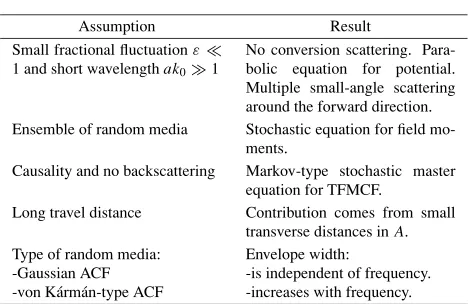
Table 1. Assumptions and results.
Assumption Result
Small fractional fluctuationε 1 and short wavelengthak01
No conversion scattering. Para-bolic equation for potential. Multiple small-angle scattering around the forward direction. Ensemble of random media Stochastic equation for field
mo-ments.
Causality and no backscattering Markov-type stochastic master equation for TFMCF.
Long travel distance Contribution comes from small transverse distances inA. Type of random media:
-Gaussian ACF -von K´arm´an-type ACF
Envelope width:
-is independent of frequency. -increases with frequency.
0a), which is practically independent of cen-tral angular frequency.
The Fourier transform of the exponential term in the RHS of Eq. (6) is
which does not influence the broadening of individual wave packets but shows the wandering effect from statistical av-eraging of the phase fluctuations of different rays. The time width of the wandering effect is proportional to the square root of travel distance. We note that lim
r→0w (r,t)=δ (t)and ∞
−∞wdt=1.
How each assumption affects the approximation and the results are summarized in Table 1.
2.2 Intensity spectral density
For P-waves, the angular-component intensity at a dis-tanceris written as an integral of the intensity spectral den-sity (ISD)IθP over central angular frequency:
where we assumed that TFMCF is independent ofθc. In a
mean square (MS) envelope. ISD can be written as a con-volution of ISD without wandering effectIP
0θand the wan-dering termwin time domain as
Here we define the reference ISD without wandering effect
IR
0 as the Fourier transform of0 2as
which is the ISD of a cylindrical scalar wave as de-rived in Fehler et al. (2000). For the derivation of the last line in Eq. (13) we used the relation 2πi ug(u) = ∞
−∞dωde−iωdu∂ωdgˆ(ωd), wheregˆis the Fourier transform
of time functiong.
Using the leading term in Eq. (3),∂rU ≈(i/2k0r2)∂θ2U, we have the radial-component intensity as
where the radial component ISDIP
r is written as a
convolu-tion of ISD without wandering effectIP
0rand the wandering
termwas
The initial condition of Eq. (8) represents the isotropic radi-ation of a wavelet characterized by a delta-fucntion for the source time function’s square per frequency:
For a given source time function’s square per angular fre-quencyi(t;ωc), we calculate the convolution
IP
θ ⊗i for
the angular component andIP
r ⊗ifor the radial component
since constituent waves are incoherent.
For the case of isotropic radiation of anS-wavelet from a point source, replacing P with S and substituting the average S-wave velocity into V0,
angular and radial component wave intensitiesIS
θ and
IS r,
Fig. 1. Temporal change inIR
0 and(t−r/V0)
IR
0/tM against reduced
timet −r/V0 for a point source radiation in random elastic media characterized by a Gaussian ACF.
0 10 20 30 40 0.04
0.3
0.2
0 0.1 0 0.02
t -1 ∝
t -1.5 ∝
Lapse Time [s]
RMS Amplitude
Radial Component Angular Component
(a)
(b)
RMS Amplitude
50km
200km 150km 100km
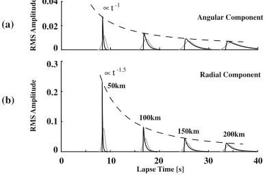
Fig. 2. Square root ISD envelopes ofP-waves for an isotropic radiation from a point source in random elastic media characterized by a Gaus-sian ACF predicted by the Markov approximation for TFMCF: (a) the angular component and (b) the radial component. Thin solid curves and gray bold curves show square root of ISDs without wandering effect and those with wandering effect, where the source time function of a 2-Hz wavelet. Broken curves show peak amplitude decays according to a power of lapse time.
2.3 Characteristics of resultant ISDs
As was done in Fehler et al. (2000), we can numeri-cally evaluate the reference ISD without wandering effect by Eq. (14) by using an Fast Fourier Transform (FFT). In Fig. 1 we plot IR
0 as a gray curve against reduced time t−r/V0. It takes the maximum value of about 3.15/(2πr tM)
at the reduced time of about 0.12tM. The peak height of
I0R is proportional to the inverse cube of travel distance since the characteristic time is proportional to the square of dis-tance. A black curve shows(t−r/V0)
I0R/tM, which has
the maximum value of about 0.49/(2πr tM)at the reduced
time of about 0.21tM, which is nearly twice the peak delay
of I0R. This means thatI0Pθ has a maximum value of about 0.31V0/r2. The peak height of
IP
0θ is nearly proportional
to the inverse cube of travel distance as IR
0 when the peak height ofI0Pθis negligible. There are constraints on the time integral of ISDs. We haver∞/V
0dt
IR
0 =1/ (2πr); however, the time integral ofIP
0θis independent of travel distance as ∞
r/V0dt
IP
0θ = ε2/
3√πa, suggesting that the time inte-gral ofIP
0θ offers a stable measure of the ratio of velocity inhomogeneity to the correlation distance.
Fig. 3. Schematic illustration of one realization of a random elastic medium characterized by a Gaussian ACF (ε=5% anda=5 km) and the configuration of a source (star) and four receiver arrays (circles) used for FD numerical simulations, where meanP- andS-wave velocities are 6 km/s and 3.46 m/s, respectively.
Fig. 4. Examples of FD simulation traces at a distance of 150 km in one realization of a random elastic medium characterized by the Gaussian ACF for the isotropic radiation of a 2-HzP-wavelet from a point source. Only every second trace is plotted.
In Fig. 2, we plot the time traces of square root ISDs, which is a more appropriate means for a comparison with RMS envelopes, whereε=5% anda =5 km and the av-erage P-wave velocity is 6 km/s. We note thatIP
0θexceeds
IR
0 as the reduced time increases, indicating a violation of the approximation. Theoretical curves are plotted only in the range of IP
0θ <
IR
0. The asymptotic peak decay curve of the angular component
IP
0θ and that of the radial
com-ponent
IP
0r are shown by power law curvest−1andt−1.5,
respectively, as plotted by broken curves.
2.4 Comparison with finite-difference simulations
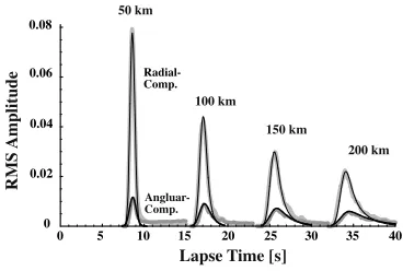
Fig. 5. Comparison of RMS envelopes of FD simulated waves (bold gray curves) and theoretical envelopes directly predicted by the Markov approximation (thin black curves) in random media characterized by a Gaussian ACF for the isotropic radiation of a 2-HzP-wavelet from the point source.
fourth-order in space. Absorbing boundary conditions are implemented at the boundaries of the computational grid. The size of the model is 450×450 km, as illustrated in Fig. 3. In the following simulation, we usedε = 5% and a =5 km. Mean P- andS-wave velocities are 6 km/s, and 3.46 km/s, respectively. The fractional fluctuation of mass density is chosen as 0.8ξ (x)according to Birch’s law (see Sato, 1984). This model is scaled to be a representative of an average crust for high-frequency seismic wave propaga-tion.
The far-field pulse shape of the outgoing P-wavelet in a homogenous medium radiated isotropically from a source located at the center is given by the convolutionur =g2⊗h, where the 2-D Green function g2(r,t) = 2V0H(V0t − r)/
V02t2−r2 (Morse and Feshbach, 1953, p. 842) is approximated as g2(r,t) ≈
√
2V0/
√
r(V0t−r)near the wave frontt≈r/V0. The source time function is given by
h(t)=c
sin Nπ T t−
N N+2sin
(N+2) π
T t
for 0≤t ≤T, (19)
whereT is the duration of the wavelet, andN is a param-eter indicating the number of maxima and minima of the wavelet. ChoosingN =2 andT =0.5 s, we have a 2-Hz wavelet with a band-limited spectrum of half-widthf be-tween 0.8 and 4.1 Hz. Around the source a homogeneous region of 1-km width is introduced to ensure pure isotropic P-wave radiation. Factorcin the source time function is chosen to satisfy0T2πr |ur|2dt=1 near the source.
The wave field is recorded at circular arrays of receivers atr =50, 100, 150 and 200 km, respectively. Each circular array consists of 72 receivers at intervals of 5◦, as shown by open circles in Fig. 3. The spatial discretization in the finite-difference (FD) scheme is 0.1 km, and the temporal dis-cretization is 6 ms, slightly below the stability limit of the numerical scheme. This choice ensures that the numerical errors remain small. The wavelength of a 2-Hz P-wavelet is smaller than the correlation distance and the medium in-homogeneity is weak.
Figure 4 shows examples of FD waveforms that have travelled 150 km through one realization of random elastic medium. Strong distortions of pulse shape and travel time
fluctuations are clearly seen. The P-wave is followed by scattered waves in the radial-component traces, and scat-tered waves also appear in the angular-component traces. We obtain the ensemble-averaged envelope at each travel distance by averaging the square of wave traces over 72 re-ceivers along the circular array in five realizations of ran-dom media, smoothing with time constant 0.5 s, and tak-ing the square root. The bold gray curves in Fig. 5 show RMS envelopes at four travel distances, clearly revealing that the peak delay and the time width of the envelope in-crease with travel distance—in both the radial and angular components. The existence of wave trains in the angular component provides clear evidence of scattering caused by random inhomogeneity. At each travel distance, the peak amplitude of the angular component is smaller than that of the radial component; however, the former amplitude de-creases more slowly than that of the latter amplitude. The peak delay of the angular component looks larger than that of the radial component.
Using ISDs with wandering effect calculated from the Markov approximation for the same parameters character-izing random media, we perform the convolution with the source time function’s square of the 2 Hz P-wavelet; then,
taking square root
IθP⊗i and
IP
r ⊗i, we obtain RMS
envelopes, where we practically put i(t) = 2πr|ur|2 of
the FD simulation near the source. Theoretical RMS en-velopes according to the Markov approximation are shown by the plots of gray curves in Fig. 2. Each envelope has a longer time width and a smaller peak height compared with the corresponding envelope without wandering effect. We find that the difference becomes smaller as the travel dis-tance increases. In Fig. 5, RMS envelopes
IP
θ ⊗i and
IP
r ⊗i predicted by the Markov approximation are
plot-ted as thin black curves together with FD envelopes. We find that the Markov approximation envelopes well explain the peak height, the delay of the peak arrival from the onset, and the envelope broadening of FD envelopes at four dis-tances. We also find a small discrepancy between them as reduced time increases at each travel distance since FD en-velopes contain large angle scattering and conversion scat-tering that the Markov approximation neglects. The impor-tance of conversion scattering for P-coda is carefully ex-amined by Przybillaet al.(2006). With the exception of the coda portion, FD envelopes are quantitatively well ex-plained by Markov envelopes.
The time integral of FD envelopes
2πr(|ur|2+ |uθ|2)dt takes nearly the same value as
that predicted from the Markov approximation at four dis-tances and the relative error is less than 2%, where the time window length is chosen as 7, 12, 18, and 24 s at 50, 100, 150 and 200 km, respectively. The ratio of time integrals of FD envelopes |uθ|2dt/ 2πr(|ur|2+ |uθ|2)dt is nearly
to 5%.
3.
Stochastic Ray Path Method
We introduce a stochastic master equation for MCF of potential field on the basis of the Markov approximation. The stochastic ray path method of Williamson (1972) uses the solution of this stochastic equation with ray travel times for the evaluation of scalar wave envelope at a given travel distance. Extending this method to vector waves, we calcu-late vector component intensities for a point source radia-tion.
3.1 Markov approximation for the MCF
For waves isotropically radiated from a point source lo-cated at the origin, we define the MCF of fieldU between different locations on the transverse line (x-axis) at a large distancer as 1(r, θ, θ, ω) ≡ U(r, θ, ω)U(r, θ, ω)∗. The MCF is a function of the difference transverse coordi-natexd ≡rθd =r(θ−θ)since it is independent of the
center of mass angleθc =(θ+θ)/2 because of isotropy
of randomness and isotropic source radiation. Neglecting backward scattering and using causality, we can derive the master equation for MCF according to the Markov approx-imation as
∂r 1+k02[A(0)−A(rθd)] 1=0, (20)
where A is the longitudinal integral of ACF as defined by Eq. (5) (see p. 244, Sato and Fehler, 1998). Integrating Eq. (20) for an incrementr, we have a solution of MCF
Using Eq. (21) successively by a split step method with an increment r, we get 1 at any distance r. The angular spectrum function (ASF) is defined as the Fourier transform of MCF in the transverse plane,
˘1(r,kx, ω)=
∞
−∞d xde
−i kxxd
1(r,xd, ω) (22)
This gives the distribution of ray wavenumbers. We may write Eq. (21) as a convolution for ASF,
˘1(r+r,kx, ω)=
where the integral kernel is
˘
(r,kx, ω)=
∞
−∞d xde
−i kxxde−k20[A(0)−A(xd)]r. (24)
The meaning of ASF becomes clear if we change the argument from wavenumber kx to local ray angle φ ≈
kx/k0 in the case of small angle scattering. Replacing
k0
where the transfer function forφis
˘ means that ray bending process is essentially governed by the spectrum of random media through function A. Ray bending is small when the wavelength is shorter than the correlation distance and velocity fluctuation is small. As travel distance increases, the incoherent term controlled by the transfer function at a small transverse distance domi-nates over the coherent term. For the envelope synthesis at a long travel distance, it is enough to use the transfer func-tion at a small transverse distance only (see, for example, Ishimaru, 1978, p. 321). For the case of Gaussian ACF, substituting Eq. (5) into Eq. (26), we have a Gaussian-type transfer function as
Intensity in the angular-frequency domain is defined by the ensemble average of the Fourier transform of displace-ment vector ˆuP(r, ω). The angular component intensity in
angular-frequency domain is given by
This can be written as an integral over local ray angleθ:
The radial-component intensity in angular-frequency do-main is given by
which is written as an integral over local ray angleφ:
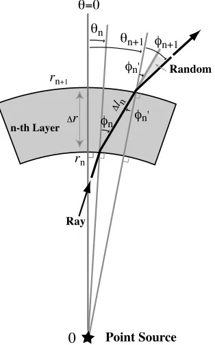
Fig. 6. Ray bending process through cylindrical layers with thicknessr
in an inhomogeneous random medium.
The isotropic radiation of coherent waves from the ori-gin is written by the initial condition 1(r →0,xd, ω) =
1/(2π), that is, ˘φ(r →0, φ, ω) = δ (φ) /(2π). When the medium is homogeneous, JP
r (rω) = 1/(2πr) and
JP
θ (rω)=0. Once ASF ˘φ is obtained in random media,
it is easy to calculate both radial and angular-component intensities JP
r and
JP
θ at a given distance from the point
source. We should note that Eqs. (29) and (31) describe stationary state.
For the case of S-waves, replacing P with S inJP r and
JθP, we have the angular and radial-component wave inten-sities in angular-frequency domain, respectively.
3.2 Cylindrical layers and ray travel times
The split-step solution - Eq. (25) - describes how rays are bent according to the velocity inhomogeneity in a layer of thickness r for stationary state. Williamson (1972) interpreted the convolution integral equation Eq. (25) as a Wiener process in that the change in ray direction is stochastically controlled by the spectrum of random media through factor A. To extend the above solution to non-stationary state problem, he used the accumulated travel time for each ray path from a source to a receiver. He proposed this method for the synthesis of scalar wave en-velopes for the case of the Gaussian transfer function. Williamson (1975) denoted this method as the stochastic ray path method, and a compact summary is given in Us-cinski (1977, Chapter 6).
The ray bending process takes place in a small region which can be well described using local Cartesian coordi-nates; however, it is necessary to use polar coordinates to describe the ray trajectory from a point source located at the origin. As illustrated in Fig. 6, we divide a random medium into many cylindrical layers with a small thickness ofr.
Fig. 7. Distribution of ray coordinate angleθand that of local ray angleφ (ASF) at three distances. The initial ray direction isθ =0 andφ=0. SD means the standard deviation.
At then-th boundary, the absolute ray location is given by ray coordinates (θn, rn), where rn is the radius from the
source,θnis the ray angle from the initial ray direction from
the sourceθ =0, and local ray angleφnis measured from
a radial direction from the source. At then +1th bound-ary after an increment of radius r in the n-th layer, the ray coordinate becomes(θn+1, rn+1), and the incident an-gle to the n +1th boundary is φn. The path length ln
satisfies lnsinφn = rn+1(θn+1−θn) and lnsinφn =
rn(θn+1−θn); that is, sinφn/sinφn =rn/ (rn+r). For
a small local ray angle, we haveφn =rnφn/ (rn+r)≈
(1−r/rn) φn. The local ray angle at then+1-th
bound-ary is bent by the medium inhomogeneity as a stochastic process, which is written by
φn+1=φn +Random≈(1−r/rn) φn+Random.
(32)
Random angles are practically generated by using the Monte Carlo method for the transfer function Eq. (27). The ray coordinate angle at then+1-th boundary then becomes
θn+1≈θn+(r/rn) φn. (33)
When the travel time of this ray at then-th boundary istn,
the travel time at then+1-th boundary becomes
tn+1=tn+
ln
V0
≈tn+
r V0
1+φ
2
n
2 . (34)
Fig. 8. Square root intensity envelopes at a distance of 100 km for isotropic radiation from a point source in 2-D random elastic media characterized by a Gaussian ACF: (a) P-wave case, (b)S-wave case. Comparison of the Markov approximation for TFMCF without wandering effect of (gray curves) and the stochastic ray path method (thin black curves).
obtained with the wandering term as given by Eqs. (12) and (16).
3.3 Coincidence of two vector envelope simulations for isotropic source radiation
For the synthesis of vector-wave envelopes for radiation from a point source, we shoot many particles from the ori-gin and calculate the travel time distribution at a given radial distance and a ray coordinate angle θ. The Monte Carlo method is used to realize the ray bending process of each particle in each cylindrical layer. Here we synthesize vec-tor envelopes in random elastic media characterized by a Gaussian ACF withε =5% anda =5 km and mean P -and S-wave velocities of 6 km/s, and 3.46 km/s, respec-tively, where the number of shots is 100,000 andr = 2 km. Figure 7 shows the distribution of ray coordinate an-gleθ and that of local ray angleφ; this distribution means that the ASF spreads with increasing travel distance for the P-waves, where the initial ray direction isθ=0 andφ=0. For the case of isotropic source radiation, we use a convo-lution of the resultant intensity and the uniform ray coordi-nate angle distribution. The thin black curves having small zigzag fluctuations in Figs. 8(a) and (b) show square root intensities calculated from the stochastic ray path method at a distance of 100 km from the P-wave source and S -wave source, respectively. The apparent duration of the S-wavelet is larger than that of P-wavelet. We plot corre-sponding solutions derived from the Markov approximation for TFMCF for comparison; these are shown as bold gray curves in Figs. 8(a) and (b). We find a good agreement be-tween vector envelopes derived from the stochastic ray path method and those derived from the Markov approximation for TFMCF for the case of isotropic radiation from a point source. The coincidence of two methods for scalar wave case in 3-D was shown by Williamson (1972).
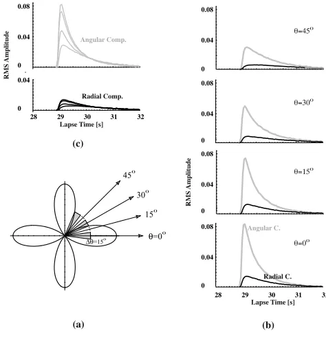
Fig. 9. Square root intensity envelopes at a distance of 100 km for a point shear dislocationS-source in 2-D random elastic media characterized by a Gaussian ACF based on the stochastic ray path method: (a) Ra-diation pattern ofS-wave intensity; (b) Square root intensity envelopes at difference azimuths; (c) Square root intensity envelopes in the radial component (solid curves) and the angular component (gray curves).
3.4 Vector wave envelopes for the case of a point shear dislocation source
The stochastic ray path method was originally developed for the case of isotropic source radiation; however, the ad-vantage of the stochastic ray path method is that it is directly applicable to nonisotropic source radiation. A point shear dislocation source is the most important nonisotropic source radiation in seismology. The radiation pattern of wave in-tensity in a plane perpendicular to the null axis is written by
(θ)=2 cos 2θ, (35)
A peak delay from the onset and a smooth decay after the peak are common to envelopes in all azimuths. We find that the difference in amplitudes between the radial and angu-lar components becomes smaller with the reduced time in-creasing at any angles. As shown in Fig. 9(c), wave ampli-tudes near the peak arrival well reflect the source radiation pattern, but the difference in amplitudes for different az-imuths diminishes as the reduced time increases in both ra-dial and angular components. These simulations give a pos-sible explanation for the observed fact that high-frequency seismograms of local earthquakes are insensitive to the fo-cal plane solution as compared with those in low frequen-cies. Observed departure from the double-couple radiation pattern at high frequencies can be explained by scattering due to medium inhomogeneity.
4.
Summary and Discussion
For the direct envelope synthesis of cylindrical vector waves in 2-D random elastic media, we have introduced two methods for the case that the medium inhomogeneity is small and the wavelength is shorter than the correlation dis-tance. Since wave conversion between P-andS-waves can be neglected, potential fields of P- and S-waves are inde-pendently governed by parabolic equations. The stochastic master equation for TFMCF of the potential field is derived using the Markov approximation. For the case of Gaus-sian ACF, taking the Fourier transform of the analytical so-lution of TFMCF, we have newly derived two-component wave envelopes. The resultant envelope of each compo-nent shows peak amplitude decay, peak delay from the on-set, and envelope broadening with increasing distance. The envelope characteristics are independent of frequency, and they are well quantified by the statistical parameters and the distance. The excitation of amplitude in the angular com-ponent forP-waves and that in the radial component forS -waves are clear evidence of scattering effect. ForP-waves, the ratio of the time integral of the square of the angular component amplitude trace to that of the square-sum of two component amplitudes with geometrical correction leads to the ratio of the MS fractional fluctuation to the correlation distance. It gives a convenient way to determine this ratio from envelope data.
We numerically studied vector wave propagation in 2-D random elastic media (meanP- andS-wave velocities of 6 km/s and 3.46 km/s, respectively) characterized by Gaus-sian ACF (ε =0.05,a =5 km) for an isotropic radiation of a 2-Hz P-wavelet by using FD simulations. At each travel distance, we take the square root of the ensemble average of the square of numerically simulated amplitude traces to calculate the RMS envelope trace of each com-ponent, which shows a good coincidence with that derived from the Markov approximation for TFMCF, with the ex-ception of the coda portion.
We next introduced the stochastic ray path method, which jointly uses the Markov approximation for MCF of the po-tential field and ray travel times. We have numerically con-firmed the coincidence of the Markov approximation for TFMCF and the stochastic ray path method for Gaussian ACF. The advantage of the stochastic ray path method is that it is directly applicable to nonisotropic source radiation.
We simulated vector wave envelopes at different azimuths for the case of a point shear dislocation source radiation. A peak delay from the onset and a smooth decay after the peak are common to envelopes in all azimuths. The differ-ence in amplitudes between the radial and angular compo-nents becomes smaller with increasing reduced time. Peak amplitudes well reflect the source radiation pattern, but the difference in amplitudes for different azimuths diminishes as reduced time increases in both radial and angular compo-nents. These results qualitatively explain the observed fact that higher frequency seismograms of local earthquakes be-come insensitive to the focal plane solution compared with lower frequency ones. When large angle scattering is neg-ligible, this method is essentially extendable for more gen-eral types of random media and a 3-D case. We are cur-rently seeking a way to simulate wave envelopes by using the Markov approximation for TFMCF for the nonisotropic source radiation case.
Acknowledgments. H. S. is supported by the grant for Scientific Research #17540389 from JSPS and the JNES open application project for enhancing the basis of nuclear safety. M. K. acknowl-edges support from the Deutsche Forschungs Gemeinschaft un-der contract KO-1068/5. Comments of Anatoly Petukhin and an anonymous reviewer were helpful for revising the manuscript.
References
Aki, K. and B. Chouet, Origin of coda waves: Source, attenuation and scattering effects,J. Geophys. Res.,80, 3322–3342, 1975.
Bal, G. and M. Moscoso, Polarization effects of seismic waves on the basis of radiative transport theory,Geophys. J. Int.,142, 571–585, 2000. Fehler, M., H. Sato, and L.-J. Huang, Envelope broadening of outgoing
waves in 2-D random media: A comparison between the Markov ap-proximation and numerical simulations,Bull. Seismol. Soc. Am.,90, 914–928, 2000.
Frankel, A. and R. W. Clayton, Finite difference simulations of seis-mic scattering: Implications for the propagation of short-period seisseis-mic waves in the crust and models of crustal heterogeneity,J. Geophys. Res., 91, 6465–6489, 1986.
Gusev, A. A. and I. R. Abubakirov, Simulated envelopes of non-isotropically scattered body waves as compared to observed ones: An-other manifestation of fractal heterogeneity,Geophys. J. Int.,127, 49– 60, 1996.
Hoshiba, M., Simulation of coda wave envelope in depth dependent scat-tering and absorption structure,Geophys. Res. Lett.,21, 2853–2856, 1994.
Ishimaru, A.,Wave Propagation and Scattering in Random Media, vols. 1 and 2, Academic, San Diego, Calif., 1978.
Korn, M. and H. Sato, Synthesis of plane vector wave envelopes in two-dimensional random elastic media based on the Markov approximation and comparison with finite-difference simulations,Geophys. J. Int.,161, 839–848, 2005.
Lee, L. C. and J. R. Jokipii, Strong scintillations in astrophysics. I. The Markov approximation, its validity and application to angular broaden-ing,Astrophys. J.,196, 695–707, 1975.
Margerin, L., M. Campillo, and B. Van Tiggelen, Monte Carlo simulation of multiple scattering of elastic waves,J. Geophys. Res.,105, 7873– 7892, DOI:10.1029/1999JB900359, 2000.
Matsumura, S., Three-dimensional expression of seismic particle motions by the trajectory ellipsoid and its application to the seismic data ob-served in the Kanto district, Japan,J. Phys. Earth,29, 221–239, 1981. Morse, P. M. and H. Feshbach,Methods in Theoretical Physics,
McGraw-Hill, Boston, 1953.
Nakahara, H., T. Nishimura, H. Sato, and M. Ohtake, Seismogram enve-lope inversion for the spatial distribution of high-frequency energy ra-diation from the earthquake fault: Application to the 1994 far east off Sanriku earthquake, Japan,J. Geophys. Res.,103, 855–867, 1998. Obara, K. and H. Sato, Regional differences of random inhomogeneities
2103–2121, 1995.
Petukhin, A. G. and A. A. Gusev, The Duration-distance relationship and average envelope shapes of small Kamchatka earthquakes,Pure Appl. Geophys.,160, 1717–1743, 2002.
Przybilla, J., M. Korn, and U. Wegler, Radiative transfer of elastic waves versus finite difference simulations in 2D random media,J. Geophys. Res.,111, B04305, doi:10.1029/2005JB003952, 2006.
Saito, T., H. Sato, and M. Ohtake, Envelope broadening of spherically outgoing waves in three-dimensional random media having power-law spectra,J. Geophys. Res.,107, doi: 10.1029/2001JB000264, 2002. Saito, T., H. Sato, and M. Ohtake, Envelope broadening of spherically
outgoing waves in three-dimensional random media having power-law spectra,J. Geophys. Res.,107, doi: 10.1029/2001JB000264, 2002. Sato, H., Energy propagation including scattering effect: Single isotropic
scattering approximation,J. Phys. Earth,25, 27–41, 1977.
Sato, H., Attenuation and envelope formation of three-component seis-mograms of small local earthquakes in randomly inhomogeneous litho-sphere,J. Geophys. Res.,89, 1221–1241, 1984.
Sato, H., Broadening of seismogram envelopes in the randomly inhomoge-neous lithosphere based on the parabolic approximation: Southeastern Honshu, Japan,J. Geophys. Res.,94, 17735–17747, 1989.
Sato, H. Synthesis of vector-wave envelopes in 3-D random elastic me-dia characterized by a Gaussian autocorrelation function based on the Markov approximation: Plane wave case,J. Geophys. Res.,111, B06306, doi:10.1029/2005JB004036, 2006.
Sato, H., Synthesis of vector-wave envelopes in 3-D random elastic me-dia characterized by a Gaussian autocorrelation function based on the Markov approximation: Spherical wave case,J. Geophys. Res.,112, B01301, doi:10.1029/2006JB004437, 2007.
Sato, H. and M. Fehler, “Seismic wave propagation and scattering in the
heterogeneous earth”, AIP Press/Springer Verlag New York, 1–308, 1998.
Scherbaum, F. and H. Sato, Inversion of full seismogram envelopes based on the parabolic approximation: Estimation of randomness and atten-uation in southeast Honshu, Japan,J. Geophys. Res.,96, 2223–2232, 1991.
Shishov, V. L., Effect of refraction on scintillation characteristics and av-erage pulsars,Sov. Astron.,17, 598–602, 1974.
Sreenivasiah, I., A. Ishimaru, and S. T. Hong, Two-frequency mutual co-herence function and pulse propagation in a random medium: An ana-lytic solution to the plane wave case,Radio Sci.,11, 775–778, 1976. Uscinski, J., The Elements of Wave Propagation in Random Media,
McGraw-Hill, New York, 1977.
Wegler, U., M. Korn, and J. Przybilla, Modeling of full seismogram en-velopes using radiative transfer theory with Born scattering coefficients,
Pure Appl. Geophys.,163, 503–531, 2006.
Williamson, I. P., Pulse broadening due to multiple scattering in the inter-stellar medium,Mon. Not. R. Astron. Soc.,157, 55–71, 1972. Williamson, I. P., The broadening of pulses due to multi-path propagation
of radiation,Proc. R. Soc. London. A.,342, 131–147, 1975.
Yomogida, K. and R. Benites, Relation between direct wave and coda : A numerical approach,Geophys. J. Int.,123, 471–483, 1995.
Yoshimoto, K., Monte Carlo simulation of seismogram envelopes in scat-tering media,J. Geophys. Res.,105, 6153–6161, 2000.
Zeng, Y., K. Aki, and T. L. Teng, Mapping of the high-frequency source radiation for the Loma Prieta earthquake, California,J. Geophys. Res., 98, 11981–11993, 1993.