R E S E A R C H
Open Access
Bayesian filtering for indoor localization and
tracking in wireless sensor networks
Anup Dhital
1,2, Pau Closas
3*and Carles Fernández-Prades
3Abstract
In this article, we investigate experimentally the suitability of several Bayesian filtering techniques for the problem of tracking a moving device by a set of wireless sensor nodes in indoor environments. In particular, we consider a setup where a robot was equipped with an ultra-wideband (UWB) node emitting ranging signals; this information was captured by a network of static UWB sensor nodes that were in charge of range computation. With the latter, we ran, analyzed, and compared filtering techniques to track the robot. Namely, we considered methods falling into two families: Gaussian filters and particle filters. Results shown in the article are with real data and correspond to an experimental setup where the wireless sensor network was deployed. Additionally, statistical analysis of the real data is provided, reinforcing the idea that in this kind of ranging measurements, the Gaussian noise
assumption does not hold. The article also highlights the robustness of a particular filter, namely the cost-reference particle filter, to model inaccuracies which are typical in any practical filtering algorithm.
1. Introduction
Wireless sensor networks (WSNs) enable a plethora of applications, from which localization of moving devices appears as an appealing feature that complements (or substitutes) global navigation satellite systems (GNSSs) based localization, especially in places where GNSS sig-nals are very weak, such as in indoor environments, or in situations where the portion of in-view sky is small, such as urban areas with tall buildings.
There is extensive literature available on the topic, see for instance [1,2] and references therein. In the last dec-ade, literally hundreds of research papers have been published dealing with localization and tracking of devices surrounded by wireless sensors, a problem that can be mathematically cast into an estimation problem of time-varying parameters, and where the equations modeling the system are essentially nonlinear. Two main types of estimation techniques have been consid-ered so far: (i) centralized approaches, in which all mea-surements obtained by the sensors are transmitted to a central processing unit in charge of performing the esti-mation (see, e.g., [3]), and (ii) distributed estiesti-mation
techniques (see [4,5]), where each sensor is responsible for the processing of its measurements and of data pro-vided by neighboring sensors. Most of the proposed solutions can be classified in the framework of Bayesian filtering, a statistical approach that has also evolved importantly during the last few years due to its good behavior in dynamical nonlinear systems [6,7] and the availability of powerful computational resources that enable their practical application. For instance, in [8] measurements were collected from various sensors and processed in a centralized processing unit wherein a particle filter was used to track a moving target. More-over, [9] showed how even measurements of different types can be incorporated into a single filtering algo-rithm. In [9], authors tracked moving objects using var-ious kinds of Bayesian filters.
From the wide range of wireless technologies available for WSNs, we focus our attention on impulse-radio-based ultra-wideband (UWB), a technology that has a number of inherent properties, which are well suited to sensor network applications. UWB technology not only has a very good time-domain resolution allowing for precise localization and tracking, but also its noise-like signal properties create little interference to other sys-tems and are resistant to severe multipath and jamming. In [10], authors provided an overview of the IEEE 802.15.4a standard, which adopts UWB impulse radio to * Correspondence: [email protected]
3Centre Tecnològic de Telecomunicacions de Catalunya (CTTC), Parc
Mediterrani de la Tecnologia, Av. Carl Friedrich Gauss 7, 08860 Castelldefels, Barcelona, Spain
Full list of author information is available at the end of the article
ensure robust data communications and precision ranging.
In this article, we undertake an experimental approach with commercial off-the-shelf devices, in contrast to most contributions where controllable, computer-simu-lated, results are used to assess the performance of a given method. Here, the focus was on the use of real-world data, with its inherent inaccuracies and non-mod-eled effects, to test a set of localization algorithms. This prevented distributed estimation techniques, since the sensor nodes did not allow additional, custom signal processing, but provided real-life ranging measurements from which interesting conclusions could be extracted, such as their non-Gaussianity nature. From an algorith-mic perspective, we analyzed a set of sequential estima-tion techniques that account for a priori informaestima-tion of the moving device, the so-called Bayesian filters. In par-ticular, Gaussian filters and particle filters were studied and compared in the nonlinear setup. The former included the well-known extended Kalman filter (EKF), and the recently proposed quadrature and cubature Kal-man-type techniques that showed a compromise between filtering performance and computational com-plexity. The class of particle filters we investigated encompassed standard and cost-reference particle filters (CRPFs). Another main contribution of this work is the assessment of the robustness of these methods to non-Gaussian model distributions as well as other model inaccuracies through the processing of real world data. Specially remarkable is the robustness performance of the CRPF, since model assumptions are mild compared to the rest of the filtering solutions.
The article is organized as follows. In Section 2, the experimental setup is described, including an statistical analysis of the database. Section 3 provides an overview of Bayesian filtering techniques, motivating the descrip-tions of suitable algorithms depending on the assump-tions about the distribution of measurement noise and the linearity of the measurement equation. Section 4 presents results of the aforementioned algorithms in the experimental scenario described in Section 2, and finally Section 5 draws some conclusions.
2. Experimental setup
The work reported in this article is related to the exten-sive UWB measurement campaign made within NEW-COM++, an EU FP7 Network of Excellence [11]. The measurement campaign was performed in an indoor environment with a network ofN= 12 static UWB sen-sors deployed in the area. The scenario was an office-like environment, whose floor map can be consulted in Figure 1. From the sensors shown in the figure, we only take into account UWB technology, neglecting thus the deployed ZigBee sensors. In this experimental setup, a
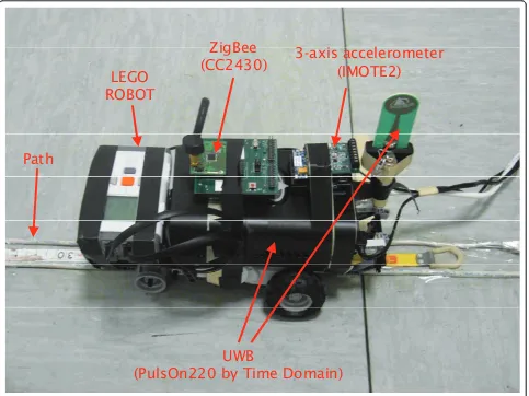
robot was moved in a straight path along the corridor of a building. The robot took a 90° turn almost at the mid-dle of its run. So the trajectory of the robot was L -shaped, 20 m length approximately. The robot was equipped with a number of sensors, namely UWB, Zig-Bee, and accelerometer measures (see Figure 2). As mentioned, only UWB technology is considered in this work. The UWB sensor mounted on the robot emitted pulsed radio signals while moving on the track. The rest of 12 UWB sensors were placed around the trajectory of the robot. Range estimates provided by each UWB sen-sor were recorded and later combined by the filtering algorithms for localization. The data were taken for two cases: once by keeping the speed of the robot constant and again by moving the robot with varying speed. The speed of the robot was controlled through commands sent from a laptop using a Bluetooth channel. The robot was kept stationary for the initial 5 s before it started to move. Since the trajectory of robot was totally con-trolled according to the command generated by writing an algorithm which defines each movement of the robot in terms of direction and speed, the true position of the robot at each instant could be easily obtained. Such ground truth was estimated using a ruler located in the path (as might be observed in Figure 2) and carefully measuring by similar means the location of anchor nodes in the plane. Of course, the precision of such ground truth was limited by the experimental nature of the measurement campaign, although the procedure is valid to extract important conclusions after data proces-sing. With the knowledge of true position of robot and anchor nodes, the true range was obtained for each anchor node in the sampling instants. Figure 3 shows the comparison of true and observed ranges for anchor node seven during the full run of the robot along its tra-jectory. It can be observed that the measurements are quite noisy as compared to the true ranges (i.e., depar-ture from the ideal line).
In this work, the tracking of a single mobile node (i.e., the robot) was considered for the experiment. However, the experiment could be easily extended for multiple moving nodes if one runs independent filters per robot in the case of self-positioning, or using more sophisti-cated data association techniques to discern among tar-gets [12-15]. The multiple target tracking setup is left for future work, focusing our attention and conclusions on the case in which measurements in [11] were recorded.
rate (500 ms in our case). These sensors are interfaced via Ethernet using the user datagram protocol (UDP) controlled from a laptop as shown in Figure 2. The loca-tions of these sensor nodes were accurately measured. Note that all nodes were located at a same height of 1.13 m, with the ceiling being at 3 m. Timedomain Pul-sON 220 UWB node computed a range estimate using a proprietary time-of-arrival (TOA) estimator, whose implementation is not public. The experiment of com-puting ranges between robot’s node and the rest of nodes was performed 700 times per pair, composing the database described in [11]. Notice that some nodes were located inside neighboring rooms and hence those mea-surements were in non-line-of-sight (NLOS) conditions for the whole (or part of the) trajectory of the robot.
More precisely, the measurement database is com-posed of (i) the accurately measured locations of each node, which will be used as thetruepositions for algo-rithms assessment. In the sequel, let us usext= [xt,yt]T to denote the 2-D position of the robot at timetandri
= [xi, yi]Tthe static coordinates of thei-th node; and (ii) the instantaneous range estimates from each node ito the robot, denoted asρˆi,t. The recorded measurements
are modeled as
ˆ
ρi,t=ρi(xt) +ni,t, i∈ {1,. . .,N}, (1)
withni,tdenoting the ranging error andri(xt) = ≜ ∥xt -ri∥the true distance from the i-th node to the robot at t.
The positioning problem is that of obtaining an esti-mate xˆt of robot’s position givenρˆi,t and ri with i Î {1,...,N}. Many positioning algorithms could be used for such problem, as those reported in [17]. For instance, to enumerate some of them, we could apply a nonlinear least squares (LS) algorithm to deal with (1), such as those proposed in [18,19]; a projection onto convex sets, reported in [20]; a transformation of the measurements could be done to obtain a linear equation [21], which can be straightforwardly solved by an LS, total LS or weighted LS algorithms. The list of algorithms is
××××
=LJ%HH$QFKRU1RGHV
××××
8:%$QFKRU1RGHV
²
7UDMHFWRU\
obviously not limited to the latter and one might find many contributions in the literature. Here, we are inter-ested in those methods that sequentially estimate the possibly time-evolving mobile position given the avail-able measurements, as well as previous records. This sequential procedure finds its theoretical justification within Bayesian filtering, which is outlined in Section 3, along with some popular filtering algorithms.
2.1. Testing for normality of UWB-based distance measurements
Before delving into the use of Bayesian filters for track-ing the mobile robot, it is important to assess the degree of Gaussianity of the measures in the database. The aforementioned database serves to test positioning algo-rithms, which sometimes resort to the Gaussian assumption, and thus their performance potentially depends on the validity of such assumption.
/(*2
52%27
=LJ%HH
&&
D[LVDFFHOHURPHWHU
,027(
3DWK
8:%
3XOV2QE\7LPH'RPDLQ
Figure 2Robot used in the experimental setup[11].
True range [m]
Observ
ed
range
[m]
2 3 4 5 6 7 8
2 3 4 5 6 7 8 9 10 11
There have been several attempts to model the indoor propagation channel for UWB transmissions. Particu-larly, a model due to [22] was proposed for the distribu-tion of TOA estimates. In this work, it was already seen that these errors could not be considered merely Gaus-sian, but of a rather more complex nature. The latter includes multipath effect (bias) and LOS/NLOS condi-tions. Recent works have reinforced this idea [23,24].
In this section, we analyze the particular results reported in [11] using the Anderson-Darling test, which is one of the most powerful tools to assess normality of a sample based on its empirical distribution function [25].
In order to provide meaningful results, from a statisti-cal point of view, a database of Lm = 700 independent measures is considered here. In this setup, the same set of UWB anchor nodes was used, with same locations, andLmrange measures were recorded for each pair of connected nodes (i, j) [11]. The Anderson-Darling test, which can be consulted in Appendix 1 and particular-ized to our application, is a detector to assess whether the set of measurements from i to jfollows a normal distribution with unknown mean and variances or not. Let us denote the probability that the test output is affirmative asPi,j{H0}, whereH0is the hypothesis that
the sample is normally distributed.
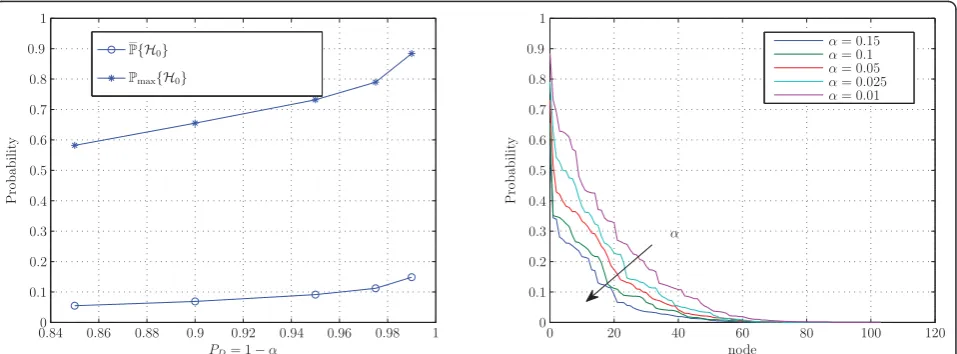
The results can be consulted in Figure 4 for different values of the detection probability. In Figure 4a, the average probability of accepting H0, P{H0}has been
plotted. It is defined as
P{H0}=
1
nc
i,j∈C
Pi,j{H0}, (2)
whereCis the subset of all nodes that are connected to others, i.e., those whose measurements are available
in the database. The dimension of C is denoted by nc= dim{C}. Notice that there are pairs which are not
connected, for instance due to obstacles in the propaga-tion path. Figure 4a also shows the maximum probabil-ity, over all nodes inCthatH0is accepted:
Pmax{H0}= max
i,j∈C Pi,j{H0}. (3) The results show that the Gaussian assumption is not realistic. Probability values below 0.15 were obtained on the average. Moreover, even in thebest measures, where the Gaussianity fits the most, probability values range from 0.582 to 0.884 depending on the significance level a. For the sake of completeness, Figure 4b plots the ordered values of Pi,j{H0}withi,j∈C. From this, we
can see that the probability decays rapidly and that actu-ally few measurements could be classified as Gaussian with a probability larger than 0.5 even with low values ofa.
As a conclusion of this subsection, we can claim that the Gaussian assumption does not hold in general for the measurements in the database [11]. Even though in some pairs of range measures it could be accepted, the majority of pairs failed the statistical test. Therefore, it is expected that those filtering algorithms based on such modeling assumption should behave poorly when com-pared with other techniques that can cope with non-Gaussianities or are distribution free.
3. Bayesian filtering
The problem of interest concerns the estimation of an unobserved discrete-time random signal in a dynamic sys-tem. The unknown is typically referred to as the state of the system. State equation models the evolution in time of states as a discrete-time stochastic function, in general
PD= 1−α
Probabilit
y
P{H0}
Pmax{H0}
0.840 0.86 0.88 0.9 0.92 0.94 0.96 0.98 1 0.1
0.2 0.3 0.4 0.5 0.6 0.7 0.8 0.9 1
Probabilit
y
node
α= 0.15
α= 0.1
α= 0.05
α= 0.025
α= 0.01
α
0 20 40 60 80 100 120 0
0.1 0.2 0.3 0.4 0.5 0.6 0.7 0.8 0.9 1
xt =ft−1(xt−1,ut), (4)
whereft-1(·) is a known, possibly nonlinear, function of
the state xtandutis referred to as process noise which gathers any mismodeling effect or disturbances in the state characterization. The relation between measure-ments and states is modeled by
yt=ht(xt,nt), (5)
where ht(·) is a known, possibly nonlinear function and ntis referred to as measurement noise. Both pro-cess and measurement noise are assumed with known statistics and are mutually independent. The initial a priori distribution of the state vector is assumed to be known, p(x0) ≜ p(x0|y0). From a theoretical point of
view, all necessary information to infer information of the unknown states resides in the posterior distribution.
Bayesian filtering involves the recursive estimation of states xt∈Rnx given measurements yt∈Rny at time t
based on all available measurements,y1:t= {y1,...,yt}. To
that aim, we are interested in the filtering distributionp (xt|y1:t) and its recursive computation givenp(xt-1|y1:t-1),
as well asp(yt|xt) and p(xt|xt-1) referred to as the
likeli-hood and the prior distributions, respectively. Such recursive solution is implemented in two steps, predic-tion and update, each one consisting in the evaluapredic-tion of integrals. The reader is referred to textbook refer-ences for further insight into the Bayesian filtering fra-mework [6,26-28]. Once the filtering distribution becomes available, one is typically interested in comput-ing statistics from it. For instance, the minimum mean square error (MMSE) estimatorEX|Y{xt|y1:t}, or in
gen-eral any function of the statesEX|Y{ϕ(xt)|y1:t}.
Unfortunately, the filtering equations involved in the Bayesian estimation can be solved analytically only in few cases such as the case of linear/Gaussian dynamic systems where the KF yields to the optimal solution [29]. In general setups, one has to resort to suboptimal solutions, most of them based on efficient numerical integration methods [6].
The experimental setup presented in Section 2 can be easily mapped into a dynamic system of the form (4)-(5). For instance, a linear constant acceleration model has been adopted for state evolution [30], and thus
⎛
where the state vector is composed of position and velocity components, pt ≜(xt, yt)T and vt ≜(ẋt, ẏt)T, respectively. Process noise utis assumed to be a
zero-mean Gaussian process, i.e., ut ∼N(0,Q), with
covar-iance chosen to beQ= 0.1 ·I4 hereinafter according to
measurement campaign processing. Finally, T denotes the sampling period in (6).
In (6) we have accounted for external information other than ranging. In particular, we have considered that the robot was equipped with an inertial measure-ment unit (IMU) that provides filtered estimates of acceleration of the mobile [31,32]. Particularly, we con-sidered the three-axis acceleration sensor LIS3L02DQ [33]. at(x¨t,y¨t)T can then be modeled as the true
acceleration plus zero-mean additive Gaussian noise with a standard deviation 0.01 m/s2.
On the other hand, from (1), we know that measure-ment equation
is nonlinear. As some of the most popular Bayesian fil-ters resort to the Gaussian assumption, we consider that measurement noisentis normally distributed according tont∼N(0,R), although we know from Section 1 that
it is not the case in general. Notice that some of the fil-ters that will be discussed in this article do not impose Gaussianity of noise distributions. In the simulation results of Gaussian filters reported in Section 4, we con-sidered thatR= 4 ·INm2. This value was obtained after off-line analysis of database measurements.
The rest of this section presents a number of filtering algorithms based on different assumptions on the model defined by (4)-(5). Particularly, we focus our attention on the location problem defined in Section 2, in which measurements were nonlinear and states evolved linearly.
3.1. Extended Kalman filter
around the mean of the relevant random variable and apply the linear KF to this linearized model. This filter behaves poorly when the degree of nonlinearity becomes high. Moreover, EKF involves the analytical derivation of the Jacobians which can get extremely complicated for complex models. In our case, measurements are defined by range estimates (1) and the Jacobian ofht, necessary for EKF implementation, is
∇xtht=
3.2. Sigma-point Kalman filters
To overcome the drawbacks of EKF, many derivatives of KF have been proposed to date, the most popular one being the unscented Kalman filter (UKF) [34]. UKF belongs to a family of Kalman-like filters, called the sigma Point Kalman filters (SPKFs) [35]. SPKF addresses the issues of EKF for nonlinear estimation problems by using the approach of numerical integration. The dynamic sys-tem is again considered Gaussian, and thus one can iden-tify that the prediction/update recursion can be transformed into a numerical evaluation of the involved integrals in the Bayesian recursion [36]. Then, only esti-mates of mean and covariance of predicted/update distri-butions are necessary and the integrals are numerically evaluated by a minimal set of deterministically chosen weighted sample points, called thesigma points. The non-linear function is then approximated by performing statis-tical linear regression between these points. This approach of weighted statistical linear regression takes into account the uncertainty (i.e., probabilistic spread) of the prior ran-dom variable. Besides UKF, various other SPKFs such as quadrature Kalman filter (QKF) [37,38] and cubature Kal-man filter (CKF) [39] have been proposed and the choice among these filters depending upon various factors such as the degree of nonlinearity, order of system state, required accuracy, etc. Moreover, computationally efficient and numerically stable variants of these filters have also been proposed by means of the square root version of QKF and CKF. Although the former is able to provide enhanced results with respect to the CKF [40], its compu-tational cost is considerably larger in high-dimensional problems. Whereas the number of sigma-points generated within the QKF increases exponentially with nx, the increase is linear in the CKF case.
3.3. Standard particle filter
All of the Kalman-type filters, discussed above, are based on the assumption that the probabilistic nature
of the system is Gaussian. The performance of these filters tend to degrade when the true density of the system is not Gaussian. With the improvement in pro-cessing power of the computers, sequential Monte Carlo (SMC) based Bayesian filters are gaining popu-larity as they intend to address the problems of non-linear systems, which do not necessarily have a Gaussian distribution. The term particle filtering (PF) denotes one of the algorithms in the SMC methods family [41,42].
As opposite to Kalman-type filters, where the poster-ior distribution is fully characterized by its mean and covariance, a PF provides a discrete characterization of the distribution. The set of Npweighted random points
is referred to as particlesx(ti),w(ti)NP
i=1. These random
samples are drawn from the importance density distri-bution,π(·),
and weighted according to
˜
Here, we consider the standard particle filter (SPF) based on the sampling importance resampling (SIR) concept [7]. In this case,π(·) =p
xtx(t−i)1
is the transi-tional prior and weights can be expressed in terms of the likelihood distribution,w˜(ti)=p
ytx(ti)
. After
parti-cle generation, weighting and normalization
, a MMSE estimate of the state can be computed as
which was proved to convergea.s. to the true value if Npwas large enough [43,44].
A typical problem of PFs is the degeneracy of particles, where all but one weight tend to zero. This situation causes the particle to collapse to a single state point. To avoid degeneracy, we apply resampling, consisting in eliminating particles with low importance weights and replicating those in high-probability regions [45,46].
xt(i)∼Nxt(−i)1,Q (13)
in this case, where we made use of the assumptions of the dynamic system described in (6)-(7).
3.4. Cost-reference particle filter
Particle filters are also sensitive to the proper specifica-tions of the model distribuspecifica-tions [47]. In fact in many situations, especially when the true noise distribution is unknown or it does not have a proper mathematical model, it is impossible to obtain a solution in closed form and hence mostly a Gaussian distribution is assumed for the ease of computation and to obtain tractable solution. So, it is likely that the PFs may degrade in performance whenever the assumed distribu-tion is different from the true distribudistribu-tion.
A new type of SMC filter, known as the CRPF, was first introduced in [48]. The idea in CRPF is to propa-gate the particles from one time epoch to the other based on some user-defined cost function. This family of methods tries to overcome some limitations of gen-eral PF algorithms: namely, the need for a tractable and realistic probabilistic model of the a priori distribution of the state, p(x0), the conditional density of the
transi-tion,p(xt|xt-1) and the likelihood distributionp(yt|xt). In
order to surmount such problems, CRPF methods per-form the dynamic optimization of an arbitrary cost function, which is not necessarily tied to the statistics of the state and the observation processes, instead of rely-ing on a probabilistic model of the dynamic system (in contrast to the SPF algorithm). By a proper selection of this cost function, we can design and implement algo-rithms in a quite simple manner, regardless of the avail-ability of process and measurement noise densities.
The CRPF algorithm can be interpreted as follows. Firstly, Np particles are randomly initialized at t= 0.
Usually, one draws from a uniform distribution in the bounded intervalIx0, and a zero cost is assigned to each particle:
cles with higher cost are selected (by resampling) and those with lower cost are rejected. The cost of the selected particles does not change in this stage.
Preserving the cost of particles after resampling helps to shift particles toward local minima of the cost function. The predictive cost of the particle, defined as
R(i)
is calculated for each particle. We use the following risk function
Then, a probability mass function (PMF) of the form
ˆ decreasing function, known as the generating function. The most intuitive choice of PMF is
μR(i)
t
= 1/R(ti), (20)
which we adopt in the sequel. Then, we resample the trajectoriesx(ti),C
The following algorithmic step is particle propagation. First, a set of Np random particles are drawn from an
arbitrary conditional distribution,pt+1(xt+1|xt), with only
constraint being that Ept+1(xt+1|xt){xt+1}=ft(xt). These new particles have associated weights
C(i)
where,l, which lies between 0 and 1, is the forgetting factor that controls the weights assigned to old observa-tions.C(t+1i) is the incremental cost function. An intui-tive and computationally simple choice [49] is
C(i)
t+1=yt+1−ht
x(t+1i)q, (22) where q ≥ 1. The updated set of particles is then
x(t+1i),Ct(+1i)Np
i=1, which is used for estimation purposes as
follows. As in the selection step, a PMF is once again defined:
ˆ
xt+1= Np
i=1
π(i)
t+1x (i)
t+1, (24)
which reminds of the estimator in (12) for the SPF algorithm.
4. Results
The Bayesian filters introduced in Section 3 were used to track and locate the robot of the experimental setup in Section 2. Recall that a robot was moved along a tra-jectory while emitting an UWB ranging signal; such sig-nal was received by a set of UWB sensors located in an office environment with known locations. The problem tackled in this article is that of a data fusion center in charge of tracking the position of the robot accounting for the measured ranges. Initial position ambiguity was modeled with a Gaussian random variable with covar-iance 10 ·I2
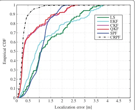
Figure 5 shows the cumulative density function (CDF) of the localization error for various filters. Also, a solu-tion based on the LS algorithm applied to the observa-tions in (7) was evaluated for the sake of comparison. Note that this is not a sequential method. Particularly, we considered Np= 50 particles for both SPF and CRPF
algorithms, as well as q = 2 for the cost function in CRPF. The plot shows the probability that a certain fil-ter occurs in an error lower than the selected x-axis value. Therefore, agoodfilter in terms of such figure of merit is one which tends quickly to 1, meaning that small errors were committed. Notice that it is a mono-tonically increasing function. From the results in Figure 5 we can see that, when applying the filters to the real data in [11], the best performance was obtained by the
CRPF. As predicted by theory, the Gaussian assumption made by the filters proved to be inappropriate, and hence the inferior performance.
The selection of the cost function for CRPF algorithm is known to be a design issue, which might modify the performance of the filter. Typically, theLq-norm is used due to its simplicity [50] as we considered in (18) and (22). For the results in Figure 5 we considered the intui-tive value q= 2, but other options are possible. In Fig-ure 5, it can also be observed that the performances of SPKFs are better than that of SPF. It shows that for cer-tain applications, SPKF can be a choice over SPF. This is especially beneficial when computational efficiency is one of the major factors under consideration. A similar result has been observed in [51], wherein a UKF has outperformed a SPF for the particular application of localization. Moreover, it can also be observed that Bayesian filters have better performance as compared to the LS estimator. This shows that using even a trivial prior information can enhance the performance, thus showing the superiority of Bayesian filters to non-Baye-sian ones. In Figure 6, the CDF of the localization error for three values ofq can be consulted. The Euclidean norm, q = 2, obtain fair results as shown in Figure 5. However, the high degree of non-Gaussianity in range measures, mainly due to the presence of a large percen-tage of outliers, makes it more appealing to use other values. For instance, it is well known [52] that the sam-ple mean (corresponding toq= 2) is less robust to out-liers than the median (q = 1). Given the relevance to our application, it was worthy to study the effect of using different types of norms in the cost function. Moreover, we studied the use ofq =∞. Results shown in Figure 6 are in accordance with theory; the valueq=
Localization error [m]
Em
pirical
CDF
LS EKF CKF QKF SPF CRPF
0 0.5 1 1.5 2 2.5 3 3.5 4 4.5 5 0
0.1 0.2 0.3 0.4 0.5 0.6 0.7 0.8 0.9 1
Figure 5Comparison of the cumulative localization error distribution functions for a number of filters.
Localization error [m]
Empirical
CDF
CRPF,q= 1
CRPF,q= 2
CRPF,q=∞
0 0.5 1 1.5 2 2.5 3 3.5 4 4.5 5 0
0.1 0.2 0.3 0.4 0.5 0.6 0.7 0.8 0.9 1
1 provides the most robust result in the presence of out-liers, being this choice for the cost function very conve-nient in the setup reported in this article.
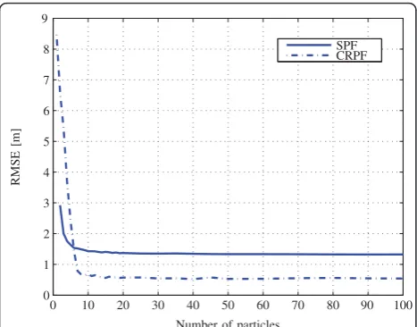
The convergence properties of SPF and CRPF do depend on the number of particles considered [43]. A number of Np-values were also tested to evaluate its
effect. Figure 7 depicts the overall root mean square error (RMSE) for SPF and CRPF algorithms versus NpÎ
[2, 100]. CRPF usedq = 1 in this figure. Apart from the conclusion that CRPF outperforms SPF, we can see that increasing Np above ten particles did not modify the
performance of both filters. The main reason could be the high noise of measures, which prevents obtaining better estimation results independently of Np.
The localization errors have been plotted with the 1.5s and 3sconfidence intervals for LS and CRPF filters in
Figure 8a.b, respectively. After using the same axis inter-vals, we can see that the error values are much less and are well bounded in the case of CRPF as compared to that of LS.
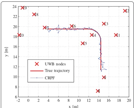
For the sake of completeness, the estimated trajectory of the CRPF with Np = 50 particles andq= 1 is shown
in Figure 9. Also the true trajectory is plotted, which started at coordinates (14.4, 11.1) meters. Crosses denote the location of UWB sensors, in accordance with the deployment in Figure 1.
5. Conclusions
In this article, we addressed the problem of robot locali-zation by means of a set of UWB ranging devices, as well as measures from acceleration sensors. In particu-lar, we used an experimental setup, and thus we dealt with real data. The contributions of this article are two-fold. On the one hand, we analyzed the Gaussian assumption of recorded data, which is commonly con-sidered in the derivation of many signal processing algo-rithms. After an exhaustive statistical analysis by the Anderson-Darling test, we found out that this assump-tion does not hold in general. Therefore, localizaassump-tion algorithms resorting to this consideration are likely to fail.
In a second part of the article, we studied a number of Bayesian filters to track the time-evolving position of the robot. Mainly, we considered Kalman-type filters, stan-dard PF, and a recently proposed CRPF, which reduces considerably model assumptions on noise distributions. From the results, with real data from the experimental setup, we saw that CRPF outperforms the rest of the fil-ters due to its inherent robustness against model inac-curacies. Other filters require rather tight model assumptions, which do not hold in general.
Number of particles
RM
SE
[m
]
SPF CRPF
0 10 20 30 40 50 60 70 80 90 100 0
1 2 3 4 5 6 7 8 9
Figure 7RMSE of localization for (a) SPF and (b) CRPF versus the number of particles, Np.
Time Epochs [secs]
Error
[m]
LS localization error
3σ 1.5σ
0 10 20 30 40 50 60 70 80 90 100 -4
-3 -2 -1 0 1 2 3
Time Epochs [secs]
Error
[m]
CRPF localization error
3σ 1.5σ
0 10 20 30 40 50 60 70 80 90 100 -4
-3 -2 -1 0 1 2 3
Appendix 1
The Anderson-Darling test for normality
The aim of the test is to assess the normality of the sample composed of a set ofLmeasured ranges between a node i and its neighbor j. The set is defined as
=1, where index ℓdenotes a realization of the
ran-dom variable (1) in the static scenario and L≤Lm. This section presents the method used to accept/reject Gaus-sianity of UWB range measures, based on the Ander-son-Darling statistic A2 as proposed in [53]. A2statistic is known to be one of the most powerful tools when testing normality [25]. The procedure is as follows.
First, for each (i, j) node pair, the set of ranges are sorted in ascending order
ˆ
and, since the hypothetic underlying normal distribu-tion is unknown, the mean and variance are estimated as
WithF(·) being the standard normal CDF,a we use the standardized sample
to compute the Anderson-Darling statistic A2, which is defined as:
Then, the null hypothesis H0that the sample is
nor-mally distributed is rejected if the modified statistic exceeds a given threshold:
A2∗A2
The threshold gais fixed for a chosen level of signifi-cancea, where 0≤a≤1 is defined as
α=PA2∗ > γα|H0
, (31)
that is, the probability of rejecting the null hypothesis while true. ga can be obtained numerically by Monte Carlo simulations or refer to the tabulated values as a function ofLanda [25]. The detection probability can then be straightforwardly computed as
PD=P
A2∗ ≤γα|H0
= 1−α. (32)
Indeed, we are not interested in the case ofL=Lmsince the Anderson-Darling test is known to reject the null hypothesis for large sample sizes in the presence of small discrepancies, such as outliers. Therefore, instead of test-ing the whole set ofLmmeasurements, the approach taken considers the random selection ofL= 10 samples from the measurement set. Notice that the test is more likely to rejectH0when increasingL. The subset is then processed
following the above procedure, which is performed inde-pendently 700 times per each pair of nodes (i, j) and aver-aged. One could use different L values with similar conclusions as those discussed in Section 1.
Endnote a
Recall that the CDF of a normal random variablexwith meanμand variances2 is(x;μ,σ2) = 1 with the error function [54] being defined as
erf(x) = √2
π ∫x0e−t
2 dt.
Acknowledgements
The authors would like to thank the anonymous reviewers for their constructive comments and suggestions, which have significantly improved the quality of this work. The authors want to acknowledge the critical contribution to the article made by their colleagues who carried out the range measurement campaign: Davide Dardari (Universita di Bologna, UNIBO), Francesco Sottile (Istituto Superiore Mario Boella), Javier Arribas (Centre Tecnologic de Telecomunicacions de Catalunya), Andrea Conti (Universit degli Studi di Ferrara), Marco Rosetti (UNIBO), Valerio Casadei (UNIBO), Sergio Contino (UNIBO), Denis Fusconi (UNIBO), and Nicolo Decarli (UNIBO). This work has been partially supported by the European Commission in the framework of the FP7 Network of Excellence in Wireless
8
COMmunications NEWCOM++ (contract n. 216715) and COST Action IC0803 (RFCSET), as well as the Spanish Science and Technology Commission TEC2008-02685/TEC (NARRA).
Author details
1Universitat Politècnica de Catalunya (UPC), Barcelona, Spain2Department of
Geomatics Engineering, University of Calgary in Calgary, Alberta, Canada 3Centre Tecnològic de Telecomunicacions de Catalunya (CTTC), Parc
Mediterrani de la Tecnologia, Av. Carl Friedrich Gauss 7, 08860 Castelldefels, Barcelona, Spain
Competing interests
The authors declare that they have no competing interests.
Received: 28 December 2010 Accepted: 19 January 2012 Published: 19 January 2012
References
1. A Boukerche (Ed.), Algorithms and Protocols for Wireless Sensor Networks, Ser, Wiley Series on Parallel and Distributed Computing, (Wiley-IEEE Press, Hoboken, NJ, 2008)
2. K Yu, I Sharp, YJ Guo, Ground-Based Wireless Positioning, ser, IEEE Press Series on Digital & Mobile Communication, (Wiley-IEEE Press, Chichester, UK, 2009)
3. X Sheng, YH Hu, Maximum likelihood multiple-source localization using acoustic energy measurements with wireless sensor networks. IEEE Trans Signal Process.53(1), 44–53 (2005)
4. F Cattivelli, CG Lopes, AH Sayed, Diffusion recursive least-squares for distributed estimation over adaptive networks. IEEE Trans. Signal Process. 56(5), 1865–1877 (2008)
5. A Gasparri, F Pascucci, An interlaced extended information filter for self-localization in sensor networks. IEEE Trans. Mobile Comput.9(10), 1491–1504 (2010)
6. Z Chen, Bayesian filtering: From Kalman filters to particle filters, and beyond, Adapt. Syst. Lab. (McMaster University, Ontario, Canada, Tech. Rep. 2003)
7. B Ristic, S Arulampalam, N Gordon, Beyond the Kalman Filter: Particle Filters for Tracking Applications, (Artech House, Boston, 2004)
8. J Ansari, J Riihijarvi, P Mahonen, Combining Particle Filtering with Cricket System for Indoor Localization and Tracking Services. Personal, Indoor and Mobile Radio Communications, 2007, in PIMRC 2007. IEEE 18th International Symposium on pp. 1–5 (2007)
9. V Fox, J Hightower, L Liao, D Schulz, G Borriello, Bayesian filtering for location estimation. Pervasive Comput. IEEE.2, 24–33 (2003) 10. J Zhang, PV Orlik, Z Sahinoglu, AF Molisch, P Kinney, UWB systems for
wireless sensor networks. Proc. IEEE.97(2), 313–331 (2009)
11. D Dardari, F Sottile (Eds.), WPR.B database: Annex of Progress Report II on Advanced Localization and positioning Techniques: Data Fusion and Applications. in Deliverable DB.3 Annex, 216715 Newcom++ NoE, WPR.B, (2009)
12. Y Bar-Shalom, E Tse, Tracking in a cluttered environment with probabilistic data association. Automatica.11, 451–460 (1975). doi:10.1016/0005-1098(75) 90021-7
13. Y Bar-Shalom, TE Fortmann, Tracking and Data Association, (Academic Press, Orlando, 1988)
14. DB Reid, An algorithm for tracking multiple targets. IEEE Trans. Automat. Contr.24(6), 443–454 (1979)
15. S Blackman, Multiple hypothesis tracking for multiple target tracking. IEEE Aerosp. Electron. Syst. Mag.19(1), 5–18 (2004)
16. Time Domain Corporation http://www.timedomain.com/ (June 2009) 17. MR Gholami, E Ström, M Rydström, Indoor sensor node positioning using
UWB range measurements, in Proc. XVII European Signal Processing Conference, EUSIPCO’09, (Glasgow, Scotland, August 2009)
18. J Ängeby, Estimating signal parameters using the nonlinear instantaneous least squares approach. IEEE. Trans. Signal Process.48(10), 2721–2732 (2000). doi:10.1109/78.869022
19. R Storn, K Price, Differential evolution—a simple and efficient adaptive scheme for global optimization over continuous spaces. J. Global Optim. 11, 341–359 (1997). doi:10.1023/A:1008202821328
20. D Blatt, AO Hero III, Energy-based sensor network source localization via projection onto convex sets. IEEE. Trans. Signal Process.54(9), 3614–3619 (2006)
21. C Meesookho, U Mitra, S Narayanan, On energy-based acoustic source localization for sensor networks. IEEE. Trans. Signal Process.56(1), 365–377 (2008)
22. B Alavi, K Pahlavan, Modeling of the TOA-based distance measurement error using UWB indoor radio measurements. IEEE Commun. Lett.10(4), 275–277 (2006). doi:10.1109/LCOMM.2006.1613745
23. N Alsindi, B Alavi, K Pahlavan, Measurement and modeling of
ultrawideband TOA-based ranging in indoor multipath environments. IEEE Trans. Veh. Technol.58(3), 1046–1058 (2009)
24. G Bellusci, GJM Janssen, J Yan, CCJM Tiberius, Modeling distance and bandwidth dependency of TOA-based UWB ranging error for positioning. Rec. Lett. Commun pp. 1–4 (2009)
25. MA Stephens, EDF statistics for goodness of fit and some comparisons. J Am. Stat. Assoc.69(347), 730–737 (1974). doi:10.2307/2286009 26. BDO Anderson, JB Moore, Optimal Filtering, (Prentice-Hall, Englewood,
1979)
27. H Sorenson, Recursive Estimation For Nonlinear Dynamic Systems, (Marcel Dekker, New York, 1988)
28. SM Kay, Fundamentals of Statistical Signal Processing. Estimation Theory, (Prentice-Hall, Upper Saddle River, 1993)
29. RE Kalman, A new approach to linear filtering and prediction problems. Trans. ASME J. Basic Eng. D.82, 35–45 (1960). doi:10.1115/1.3662552 30. F Gustafsson, F Gunnarsson, N Bergman, U Forssell, J Jansson, R Karlsson, PJ
Nordlund, Particle filters for positioning, navigation and tracking. IEEE. Trans. Signal Process.50(2), 425–437 (2002). doi:10.1109/78.978396
31. MS Grewal, LR Weill, AP Andrews, Global Positioning Systems, Inertial Navigation, and Integration, 2nd edn., (Wiley, Hoboken, 2007)
32. D Groves, Principles of GNSS. Inertial and Multisensor Navigation Systems, (Artech House, London, England, 2008)
33. 3-axis acceleration chip LIS3L02DQ datasheet, STMicroelectronics. http:// www.datasheetcatalog.org/datasheet2/1/036ete1wq40k5kgkoi91389ap83y. pdf (2005)
34. S Julier, J Uhlmann, HF Durrant-White, A new method for nonlinear transformation of means and covariances in filters and estimators. IEEE Trans. Automat. Contr.45, 477–482 (2000). doi:10.1109/9.847726 35. RVD Merwe, E Wan, Sigma-point Kalman filters for probabilistic inference in
dynamic state-space models, Proceedings of the Workshop on Advances in Machine Learning, (Montreal, Canada, 2003)
36. K Ito, K Xiong, Gaussian filters for nonlinear filtering problems. IEEE Trans. Automat. Contr.45(5), 910–927 (2000). doi:10.1109/9.855552
37. I Arasaratnam, S Haykin, RJ Elliot, Discrete-time nonlinear filtering algorithms using Gauss-Hermite quadrature. Proc IEEE.95(5), 953–977 (2007) 38. I Arasaratnam, S Haykin, Square-root quadrature Kalman filtering. IEEE Trans.
Signal Process.56(6), 2589–2593 (2008)
39. I Arasaratnam, S Haykin, Cubature Kalman filters. IEEE Trans. Autom. Control. 54(6), 1254–1269 (2009)
40. C Fernández-Prades, J Vilà-Valls, Bayesian nonlinear filtering using quadrature and cubature rules applied to sensor data fusion for positioning, in Proc. of the IEEE International Conference on Communications, ICC’10, (Cape Town, South Africa, 2010)
41. S Arulampalam, S Maskell, N Gordon, T Clapp, A tutorial on particle filters for online nonlinear/non-Gaussian Bayesian tracking. IEEE Trans. Signal Process.50(2), 174–188 (2002). doi:10.1109/78.978374
42. PM Djurić, JH Kotecha, J Zhang, Y Huang, T Ghirmai, MF Bugallo, J Míguez, Particle filtering. IEEE Signal Process Mag.20(5), 19–38 (2003). doi:10.1109/ MSP.2003.1236770
43. D Crisan, A Doucet, A survey of convergence results on particle filtering for practitioners. IEEE Trans. Signal Process.50(3), 736–746 (2002). doi:10.1109/ 78.984773
44. X Hu, T Schön, L Ljung, A basic convergence result for particle filtering. IEEE Trans. Signal Process.56(4), 1337–1348 (2008)
45. M Bolić, P Djurić, S Hong, Resampling algorithms for particle filters: A computational complexity perspective. EURASIP J Appl. Signal Process.15, 2267–2277 (2004)
47. PM Djurić, MF Bugallo, P Closas, J Míguez, Measuring the robustness of sequential methods, in Proc. of the IEEE International Workshop on Computational Advances in Multi-Sensor Adaptive Processing, CAMSAP’09, (Aruba (Dutch Antilles), 2009)
48. J Míguez, MF Bugallo, PM Djurić, A new class of particle filters for random dynamic systems with unknown statistics. EURASIP J. Appl. Signal Process. 2004(15), 2278–2294 (2004). doi:10.1155/S1110865704406039
49. J Míguez, Analysis of selection methods for cost-reference particle filtering with applications to maneuvering target tracking and dynamic
optimization. ELSEVIER Digit. Signal Process.17, 787–807 (2007) 50. M Bugallo, J Míguez, P Djurić, Positioning by cost reference particle filters:
study of various implementations. International Conference on Computer as a Tool, EUROCON 2005, vol. 2 1610–1613 (2005)
51. N Bellotto, Hu H, Computationally Efficient Solutions for Tracking People with a Mobile Robot: An Experimental Evaluation of bayesian Filters, (Springer, Berlin, 2009)
52. PJ Huber, Robust Statistics, 2nd eds., (Wiley, New York, 1981) 53. TW Anderson, DA Darling, Asymptotic theory of certain goodness-of-fit
criteria based on stochastic processes. Ann. Math. Stat.23(2), 730–737 (1952)
54. J Proakis, M Salehi, Communciation Systems Engineering, (Prentice-Hall, Upper Saddle River, 1994)
doi:10.1186/1687-1499-2012-21
Cite this article as:Dhitalet al.:Bayesian filtering for indoor localization and tracking in wireless sensor networks.EURASIP Journal on Wireless Communications and Networking20122012:21.
Submit your manuscript to a
journal and benefi t from:
7Convenient online submission
7Rigorous peer review
7Immediate publication on acceptance
7Open access: articles freely available online
7High visibility within the fi eld
7Retaining the copyright to your article
![Figure 1 L-shaped trajectory of the robot along with the location of UWB sensors [11].](https://thumb-us.123doks.com/thumbv2/123dok_us/957294.1117183/3.595.56.542.89.452/figure-l-shaped-trajectory-robot-location-uwb-sensors.webp)