R E S E A R C H
Open Access
Analysis of the equilibrium points of
background neural networks with uniform
firing rate
Fang Xu
1*, Lingling Liu
2and Jianying Xiao
2*Correspondence:
matxufang@163.com
1Department of Mathematics,
Sichuan University, Chengdu, Sichuan 610064, China Full list of author information is available at the end of the article
Abstract
In this paper, we give a complete analysis of the equilibrium points of background neural networks with uniform firing rates. By using continuity, monotonicity of some functions and Rolle’s theorem, the number of equilibrium points and their locations are obtained. Moreover, some novel sufficient conditions are given to guarantee the stability of the equilibrium points for the network model by utilizing Taylor’s theorem. A simulation example is conducted to illustrate the theories developed in this paper.
Keywords: equilibrium point; Rolle’s theorem; background neural networks
1 Introduction
Dynamical analysis is one of the most important issues of recurrent neural networks and many results on this topic have been reported in the literature; see Atteneave []; Cohen
and Grossberg []; Forti []; Hahnloser []; Zenget al.[]; Zeng and Wang []; Cao and
Wang []; Chenet al.[]; Chen []; Tanget al.[]; Zhanget al.[]; Zuoet al.[]; Zhang
et al.[]; Li and Cao []; Samidurai and Manivannan [] and the references therein. It is also an essential step towards successful applications such as signal processing and prob-lem optimization. Analysis of the equilibrium point for the concerned recurrent neural
networks is a very important part of dynamical analysis (Chenget al.[]; Quet al.[]).
Especially, existence and stability problems of the equilibrium points for various types of recurrent neural networks have attracted significant attention of many researchers
(Mani-vannanet al.[]; Nie and Cao []; Manivannanet al.[]). Generally, two ways are used
to prove the existence of equilibria for a neural network model. One way to prove this is by using a mapping derived from the neural network being a homeomorphism (Forti and Tesi []; Chen []; Lu []; Zhao and Zhu []). Another way uses Brouwer’s fixed-point theorem (Forti []; Forti and Tesi []; Guo and Huang []; Wang []; Miller and Michel []).
In order to interpret the phenomena and exhibit how the dynamical states of recurrent neural networks are affected by a given external background input, the background neural network model was proposed in Salinas []. By utilizing theoretical models and computer simulations, it has been shown that small changes in this model may shift a network from a relatively quiet state to some other state with highly complex dynamics.
As far as we are concerned, few references have studied the dynamical properties of the
background neural network model; see Zhang and Yi []; Wanet al.[]; Xu and Yi [].
However, since the network equations (.) are nonlinear and coupled equations, neither the well-known homeomorphism method nor Brouwer’s fixed-point theorem can be used to easily investigate the equilibrium point of (.). The only known theoretical results in the literature of local stability conditions of the equilibria for background neural networks are obtained by computing eigenvalues at equilibria (Salinas []). Unfortunately, so far, the equilibrium analysis problem for the background neural networks with firing rate (the uniform firing rate means that the firing rate is the same for all neurons) remains far from completion. The major difficulty stems from the network model which consists of highly nonlinear coupled equations. The lack of basic information on equilibria creates some difficulties in discussing dynamical properties and bifurcations of the background neural networks.
In this paper, we give a complete analysis of the equilibrium for the background neu-ral networks with uniform firing rate. For the first time, we transform the equilibrium problem of the background neural network with firing rate into a root problem of a cu-bic equation. Not following the common idea of computing roots of the cucu-bic equation, we analyze the equilibria through a geometrical formulation of the parameter conditions of the background neural networks. Correspondingly, the number and coordinates of the equilibria are determined by using continuity and monotonicity, together with Rolle’s the-orem. Furthermore, novel sufficient stability conditions for the equilibria are given. The studies based on the background neural network with uniform firing rate provide an in-sightful understanding of the computational performance of system (.).
The rest of this paper is organized as follows. In Section , preliminaries are given. In Section , we establish conditions for the exact number of equilibria for the background networks. Locations of these equilibria are obtained. Moreover, we formulate novel suf-ficient conditions for stability of such equilibria. In Section , a simulation example is presented to illustrate the theoretical results. In Section , conclusions are drawn.
2 Preliminaries
The background neural network model is described by the following system of nonlinear differential equations:
τx˙i(t) = –xi(t) +
(jwijxj(t) +hi)
s+vjxj(t) (i= , . . . ,n), (.)
fort≥, wherexidenotes the activity of neuroni,hirepresents its external input,wij
rep-resents the excitatory synaptic connection from neuronjto neuroni,vis the inhibitory
synaptic connection by which a neuron decreases another neuron’s gain,τ is a time
con-stant, andsis a saturation constant. All these quantities are always positive or zero. If the
firing rate is the same for all neurons, then the network equations (.) are reduced to a nonlinear equation as follows:
τx˙(t) = –x(t) +(wtotx(t) +h)
s+vNx(t) , (.)
for allt≥.xdenotes the uniform firing rate,wtotdenotes the excitatory synaptic
For simplicity, we consider system (.) in the following equivalent form:
˙
x(t) = –x(t) +(ax(t) +b)
+cx(t) :=F(x). (.)
Herein, letτ= ,a=w√tot
s > ,b= h
√
s> ,c= vN
s > .
An equilibrium of network (.) is described as follows:
Fx∗:=–x
∗( +cx∗) + (ax∗+b)
+cx∗ = .
Let
P(x) := –x(t) +cx(t)+ax(t) +b
= –cx(t) +ax(t) + (ab– )x(t) +b,
i.e.,
F(x) = P(x) +cx.
We supposex() > and
x(t) =x()e–t+
t
e–(t–θ)(wtotx(θ) +h)
s+vNx(θ) dθ> .
It means that the trajectory of system (.) is positive. From reference Zhang and Yi [], we have
x(t) <x() +w
tot vN +
h
s + =x() + a
c +b + .
Denote
=x() +a
c +b + .
Because +cx(t) > , the equilibria of system (.) are determined by zeros ofP(x) in the
intervalI:= (,).
3 Equilibria and qualitative properties
In this section, we present novel sufficient conditions which guarantee the existence and the number of equilibria for network (.). Our approach is based on a geometrical obser-vation. We also establish stability criteria of these equilibria through the Taylor expansion at some equilibrium.
Table 1 The number of equilibria and their locations Next, we will discuss the zeros of
P(x) := –cx+ax+ (ab– )x+b (a> ,b> ,c> ).
In order to state our results easily, we partition the parameter conditions ensuring the number and locations of equilibria into the following subregions:
The derivativeP(x) = –cx+ ax+ ab– = has two zeros:
c . Consider the discriminant
P(x)of a polynomialPwith degree
P(x):=a+ c(ab– ).
We separately discuss the three cases:P(x)> ,P(x)= andP(x)< .
Case:P(x)=a+ c(ab– ) > ,i.e.,wtot+ vNwtoth– vNs> . However, ab– may
be positive, negative or zero. Thus, according to the sign of ab– , we need to discuss the
following three subcases.
simple computation, we obtainζ+<. According to Rolle’s theorem and the
Figure 1 Phas one, two or three zeros in subcase 1.1.
Figure 2 Phas one zero in subcases 1.2 and 1.3.
P(x) has a multiple one ac of multiplicity . ac is not the extreme point ofP(x). Com-bining with (.),P(x) has a positive zerox∈(,), which implies that system (.) has
a unique equilibriumE():x∗∈(,).
Case:P(x)=a+ c(ab– ) < ,i.e.,wtot+ vNwtoth– vNs< .
P(x) has no real zero. It means thatP(x) has no extreme point. By (.),P(x) is a strictly monotonically decreasing function. Thus,P(x) has a positive zerox∗∈(,). System (.) accordingly has a unique equilibriumE():x∗∈(,).
The proof is completed.
Remark It should be noted that, as shown in the proof of Theorem , we separately discuss the existence and the number of the equilibria in three cases based on the sign of
the discriminantP(x). We have employed continuity and monotonicity of the function
P(x), combined with Rolle’s theorem, to estimate the coordinates and the number of the
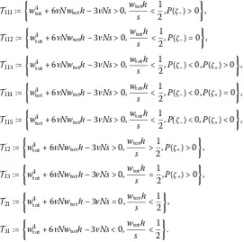
theo-Table 2 Stability of the equilibrium points for (2.3)
Conditions Equilibria (stability)
T111 E(1)1 (asymptotically stable)
T112 E(1)2 (unstable),E(1)3 (asymptotically stable)
T113 E(1)4 (asymptotically stable),E (1)
5 (unstable),E (1)
6 (asymptotically stable) T114 E(1)7 (asymptotically stable),E
(1)
8 (asymptotically stable) T115 E(1)9 (asymptotically stable)
T12 E(1)10(asymptotically stable)
T13 E(1)11(asymptotically stable)
T21 E(2)1 (asymptotically stable)
T31 E(3)1 (asymptotically stable)
rem. Moreover, these results may provide important theoretical foundations to further analyze the limit cycle and bifurcations of networks (.).
Next, we will discuss stability of the equilibrium point of system (.) by utilizing the Taylor expansion.
Theorem The stability of the equilibrium points of system(.)is described in Table.
Proof Letx∗be a general equilibrium of system (.).
The Taylor expansion ofF(x) at equilibriumx∗is described by
˙
x(t) =Fx∗+Fx∗x–x∗+Ox–x∗. (.)
SinceF(x) = +P(cxx), we have
F(x) =P
(x)( +cx) – cxP(x)
( +cx) .
DenoteQ(x) =P(x)( +cx) – cxP(x), thus
F(x) = Q(x) ( +cx).
ThenF(x∗) = Q(x∗)
(+cx∗) =
P(x∗)(+cx∗)
(+cx∗) (sinceP(x
∗) = ). The sign ofF(x∗) is the same as that
ofP(x∗), since +cx∗> .
BecauseF(x∗) = , the sign ofx˙(t) is the same as that ofF(x∗). Therefore, the stability of the equilibrium is determined by the sign ofP(x∗). Concretely,P(x) is monotonically de-creasing in (ζ+,) andP(x∗) < . Thus, the equilibrium pointE
()
is asymptotically stable.
Similarly, equilibriaE() ,E() ,E() ,E() ,E(),E(),E(),E() andE()are asymptotically stable, becauseP(x∗i) < , wheni= , , , , , , , , .
P(x) is monotonically increasing in (ζ+,) andP(x)∗> , which means that equilibrium
pointE() is unstable.
IfP(x∗) = , then the Taylor expansion ofP(x) at equilibriax∗is
˙
x(t) =Fx∗x–x∗+Ox–x∗,
F(x) = Q
(x)( +cx)–Q(x)·( +cx)·cx
( +cx) ,
whereQ(x) =P(x)( +cx) +P(x)·cx–P(x)·cx–P(x)·c. Thus, we obtain
Qx∗=Px∗ +cx∗+Px∗·cx∗–Px∗·cx∗–Px∗·c.
SinceP(x∗) = ,P(x∗) = , we haveQ(x∗) =P(x∗)( +cx∗) andQ(x∗) =P(x∗)( +cx∗) – cx∗P(x∗) = .
Therefore, we get
Fx∗=Q
(x∗)( +cx∗
)–Q(x∗)·( +cx∗)·cx∗
( +cx∗)
=Q
(x∗)( +cx∗
)
( +cx∗)
=P
(x∗)( +cx∗
) ( +cx∗) .
It means that the sign ofF(x∗) is the same as that ofP(x∗) because +cx∗> .P(ζ–) =
andP(ζ+) = at equilibriaE() :ζ–,E():ζ+, respectively. Thus,F(ζ–) = ,F(ζ+) = . P(ζ–) > because the graph ofP(x) is concave down in the neighborhood ofE().P(ζ–) =
,P(ζ–) > , thusE()is unstable. Similarly,P(ζ+) < because the graph ofP(x) is convex
up in the neighborhood ofE().P(ζ+) = ,P(ζ+) < , thusE() is asymptotically stable.
The proof is completed.
Remark It should be mentioned that we have derived the conditions for stability of the equilibria by using the Taylor expansion. In Figures and , we see that the equilibrium
is stable or unstable according to the signP(x∗) at equilibriumx∗. The method is
eas-ier and more convenient than constructing suitable Lyapunov-Krasovskii functionals or constructing energy functions.
4 Simulations
In this section, one example will be provided to illustrate and verify the theoretical results obtained in the above sections.
Example Case : Consider a class of background neural networks (.) with wtot =
.,h= .,vN= . ands= . Thus, we obtain wtot
vN + h
s + = .. We
randomly select the initial pointx()∈(, ).
Here, the parameters satisfy our conditions in Theorem : P(x)= . > ,ab=
. <.
By simple computation, equationP(x) = –cx+ ax+ ab– = is found to have two
distinct rootsζ–= .,ζ+= ., withP(ζ–) = –. < ,P(ζ+) = . > .
(a,b,c)∈T, thus, system (.) has three equilibria E() :x∗∈(, .),E () :x∗∈
(., .) andE():x∗∈(., .). According to Theorem ,E()andE()
are asymptotically stable, andE() is unstable. Figure demonstrates the theoretical
re-sults.
Figure 3 The locations and stability of equilibria of the network (2.3) withwtot= 1.8965,h = 4.6457,vN= 0.0900 ands= 50.
Figure 4 The locations and stability of the equilibrium pointE(2)1 of the network (2.3) with
wtot= 1.2,h= 12,vN= 0.02 ands= 63.36.
stable equilibrium points or periodic orbits are accompanied by the existence of contin-uous attractors. Contincontin-uous attractors have been found in many applications, including applications related to visual perception, visual images, eye memory, etc. The existence of
unstable equilibria is essential in winner-take-all problems (Yiet al.[]). Therefore, the
proposed work in this manuscript can be applied in aforementioned applications.
Case: Ifwtot= .,h= ,vN = . ands= ., then w
tot
vN + h
s + = .. We
randomly select the initial pointx()∈(, ).
In this caseP(x)= , so it follows from Theorems and that system (.) has a unique
equilibrium pointE() :x∗∈(, .), and it is asymptotically stable. The location and stability of the equilibrium points of this system are illustrated in Figure .
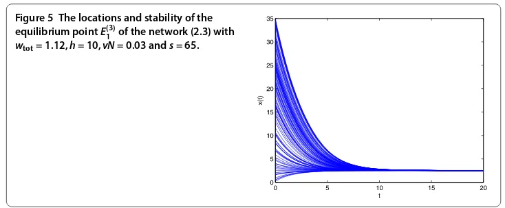
Case: Ifwtot= .,h= ,vN= . ands= , then w
tot
vN + h
s + = .. We
ran-domly select the initial pointx()∈(, ).
In this case P(x) < , so system (.) has a unique equilibrium point E() : x∗ ∈
(, .) and it is asymptotically stable. The results are shown in Figure .
In cases and , the network (.) has a unique equilibrium point which is stable. Such convergent behavior is called ‘monostability’. Monostable networks can be used to solve optimization problems. Under some conditions, the network (.) in this paper is a monostable neural network. Therefore, the proposed work provides a novel model with respect to optimization problems.
5 Conclusions
Figure 5 The locations and stability of the equilibrium pointE(3)1 of the network (2.3) with
wtot= 1.12,h= 10,vN= 0.03 ands= 65.
the conditions for the number and locations of the equilibria of the network were inves-tigated. Secondly, the conditions for stability of the equilibria were derived. The paramet-ric relations between the dynamical properties of the equilibria and network parameters were revealed. These theories are primarily based on an observation on the geometric
structures of the equationsP(x) = . These studies enrich the analytical results for the
equilibrium points of other related work.
The studies based on the background neural networks with firing rate (the uniform fir-ing rate means that the firfir-ing rate is the same for all neurons, thus, we can regard system (.) as one-dimensional) may be further developed for the studies on general
higher-dimensional systems,e.g., the mathematical methods in this paper can be applied to
an-alyze the equilibria of background neural networks with two subnetworks which exhibit
rival states (i.e., D background neural networks). The rivaling steady states have
signif-icant meaning in the development of practical applications of D neural networks. This
switch problem (Terman and Rubin []; Tothet al.[]) and binocular rivalry (Shpiro
et al.[]) are interesting topics for further research. Many practical problems, such as mechanical design and electrical networks, can be formulated as switch problems. In re-cent years, dynamical analysis for switched systems have attracted considerable research
interest (Caoet al.[]; Syed Aliet al.[]). Our manuscript has given us further insight
into providing parameter conditions for switched systems.
Acknowledgements
This work was supported in part by the National Science Foundation of China under Grant 61202045, Grant 11501475, and in part by the Program of Science and Technology of Sichuan Province of China under Grant No. 2016JY0067.
Competing interests
The authors declare that they have no competing interests.
Authors’ contributions
All authors contributed equally to the writing of this paper. All authors read and approved the manuscript.
Author details
1Department of Mathematics, Sichuan University, Chengdu, Sichuan 610064, China.2School of Science, Southwest
Petroleum University, Chengdu, Sichuan 610050, China.
Publisher’s Note
Springer Nature remains neutral with regard to jurisdictional claims in published maps and institutional affiliations.
Received: 29 May 2017 Accepted: 18 August 2017
References
2. Cohen, MA, Grossberg, S: Absolute stability of global pattern formation and parallel memory storage by competitive neural networks. IEEE Trans. Syst. Man Cybern.13, 815-826 (1983)
3. Forti, M: On global asymptotic stability of a class of nonlinear systems arising in neural network theory. J. Differ. Equ.
113, 246-264 (1994)
4. Hahnloser, RLT: On the piecewise analysis of networks of linear threshold neurons. Neural Netw.11, 691-697 (1998) 5. Zeng, Z, Wang, J, Liao, X: Global exponential stability of a general class of recurrent neural networks with
time-varying delays. IEEE Trans. Circuits Syst. I, Fundam. Theory Appl.50(10), 1353-1358 (2003)
6. Zeng, Z, Wang, J: Multiperiodicity and exponential attractivity evoked by periodic external inputs in delayed cellular neural networks. Neural Comput.18(4), 848-870 (2006)
7. Cao, J, Wang, J: Global asymptotic stability of a general class of recurrent neural networks with time-varying delays. IEEE Trans. Circuits Syst. I, Fundam. Theory Appl.50(1), 34-44 (2003)
8. Chen, T, Lu, W, Chen, G: Dynamical behaviors of a large class of general delayed neural networks. Neural Comput.
17(4), 949-968 (2005)
9. Chen, Y: Global asymptotic stability of delayed Cohen-Grossberg neural networks. IEEE Trans. Circuits Syst. I, Regul. Pap.53(2), 351-357 (2006)
10. Tang, HJ, Tan, KC, Zhang, W: Cyclic dynamics analysis for networks of linear threshold neurons. Neural Comput.17(1), 97-114 (2005)
11. Zhang, L, Yi, Z, Yu, J: Multiperiodicity and attractivity of delayed recurrent neural networks with unsaturating piecewise linear transfer functions. IEEE Trans. Neural Netw.19(1), 158-167 (2008)
12. Zuo, Z, Yang, C, Wang, Y: A new method for stability analysis of recurrent neural networks with interval time-varying delay. IEEE Trans. Neural Netw.21(2), 339-344 (2010)
13. Zhang, H, Wang, Z, Liu, D: A comprehensive review of stability analysis of continuous-time recurrent neural networks. IEEE Trans. Neural Netw. Learn. Syst.25(7), 1229-1262 (2014)
14. Li, R, Cao, J: Dissipativity analysis of memristive neural networks with time-varying delays and randomly occurring uncertainties. Math. Methods Appl. Sci.39(11), 2896-2915 (2016)
15. Samidurai, R, Manivannan, R: Delay-range-dependent passivity analysis for uncertain stochastic neural networks with discrete and distributed time-varying delays. Neurocomputing185(12), 191-201 (2016)
16. Cheng, C, Lin, K, Shin, C: Multistability in recurrent neural networks. SIAM J. Appl. Math.66(4), 1301-1320 (2006) 17. Qu, H, Yi, Z, Wang, X: Switching analysis of 2-D neural networks with nonsaturating linear threshold transfer functions.
Neurocomputing72, 413-419 (2008)
18. Manivannan, R, Mahendrakumar, G, Samidurai, R, Cao, J, Alsaedi, A: Exponential stability and extended dissipativity criteria for generalized neural networks with interval time-varying delay signals. J. Franklin Inst.354(11), 4353-4376 (2017)
19. Nie, X, Cao, J: Existence and global stability of equilibrium point for delayed competitive neural networks with discontinuous activation functions. Int. J. Syst. Sci.43(3), 459-474 (2012)
20. Manivannan, R, Samidurai, R, Cao, J, Alsaedi, A, Alsaadi, FE: Global exponential stability and dissipativity of generalized neural networks with time-varying delay signals. Neural Netw.87, 149-159 (2017)
21. Forti, M, Tesi, A: New conditions for global stability of neural networks with application to linear and quadratic programming problems. IEEE Trans. Circuits Syst. I, Fundam. Theory Appl.42(7), 354-366 (1995)
22. Lu, H: On stability of nonlinear continuous-time neural networks with delays. Neural Netw.13(10), 1135-1143 (2000) 23. Zhao, W, Zhu, Q: New results of global robust exponential stability of neural networks with delays. Nonlinear Anal.,
Real World Appl.11(2), 1190-1197 (2010)
24. Guo, S, Huang, L: Stability analysis of Cohen-Grossberg neural networks. IEEE Trans. Neural Netw.17(1), 106-117 (2006)
25. Wang, L: Stability of Cohen-Grossberg neural networks with distributed delays. Appl. Math. Comput.160(1), 93-110 (2005)
26. Miller, RK, Michel, AN: Ordinary Differential Equations. Academic Press, New York (1982)
27. Salinas, E: Background synaptic activity as a switch between dynamical states in a network. Neural Comput.15, 1439-1475 (2003)
28. Zhang, L, Yi, Z: Dynamical properties of background neural networks with uniform firing rate and background input. Chaos Solitons Fractals33(3), 979-985 (2007)
29. Wan, M, Gou, J, Wang, D, Wang, X: Dynamical properties of discrete-time background neural networks with uniform firing rate. Math. Probl. Eng.2013(1), 289-325 (2013)
30. Xu, F, Yi, Z: Convergence analysis of a class of simplified background neural networks with two subnetworks. Neurocomputing74(18), 3877-3883 (2011)
31. Yi, Z, Heng, PA, Fung, PF: Winner-take-all discrete recurrent neural networks. IEEE Trans. Circuits Syst. II47, 1584-1589 (2000)
32. Terman, D, Rubin, JE, Yew, AC, Wilson, CJ: Activity patterns in a model for the subthalamopallidal network of the basal ganglia. J. Neurosci.22(7), 2963-2976 (2002)
33. Toth, LJ, Assad, JA: Dynamic coding of behaviourally relevant stimuli in parietal cortex. Nature415, 165-168 (2002) 34. Shpiro, A, Morenobote, R, Rubin, N, Rinzel, J: Balance between noise and adaptation in competition models of
perceptual bistability. J. Comput. Neurosci.27(1), 37-54 (2009)
35. Cao, J, Rakkiyappan, R, Maheswari, K, Chandrsekar, A: ExponentialH∞filtering analysis for discrete-time switched neural networks with random delays using sojourn probabilities. Sci. China, Technol. Sci.59(3), 387-402 (2016) 36. Syed Ali, M, Saravanan, S, Cao, J: Finite-time boundedness,L2-gain analysis and control of Markovian jump switched